11.5 Efficient portfolios with two risky assets and a risk-free asset
Now we expand on the previous results by allowing our investor to form portfolios of assets \(A\), \(B\) and T-bills. The efficient set of portfolios in this case will still be a straight line in (\(\mu_{p},\sigma_{p})\)-space with intercept \(r_{f}\). The slope of the efficient set, the maximum Sharpe ratio, is such that it is tangent to the portfolio frontier constructed just using the two risky assets \(A\) and \(B\). Figure 11.8 illustrates why this is so.
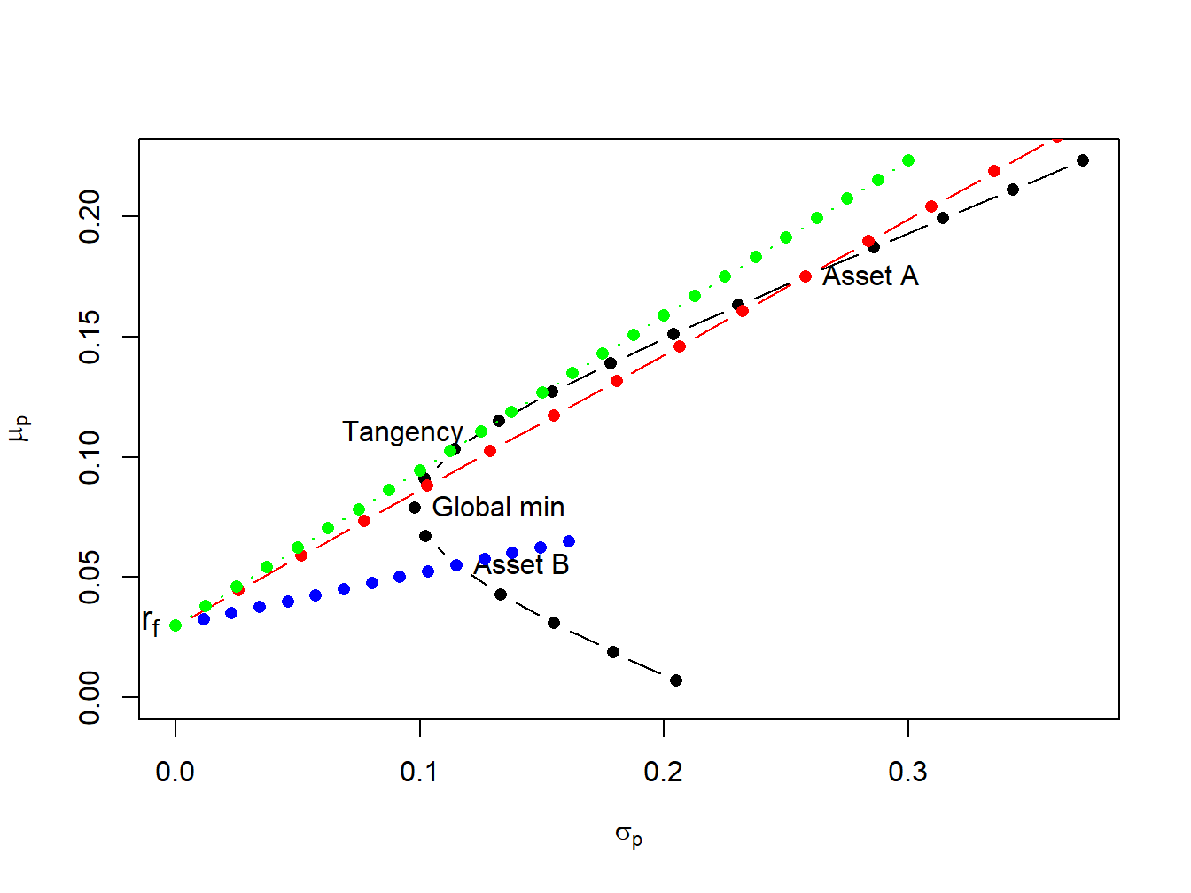
Figure 11.8: Efficient portfolios of two risky assets and T-bills. Black dots represent portfolios of assets A and B; blue dots represent portfolios of T-bills and asset B; red dots represent portfolios of T-bills and asset A; green dots represent portfolios of the tangency portfolio and T-bills.
If we invest in only in asset \(B\) and T-bills then the Sharpe ratio is \(\mathrm{SR}_{B}=\frac{\mu_{B}-r_{f}}{\sigma_{B}}=0.217\), and the CAL intersects the set of risky asset portfolios at point \(B\). This is clearly not the efficient set of portfolios. For example, we could do uniformly better if we instead invest only in asset \(A\) and T-bills. This gives us a Sharpe ratio of \(\mathrm{SR}_{A}=\frac{\mu_{A}-r_{f}}{\sigma_{A}}=0.562\), and the new CAL intersects the set of risky asset portfolios at point \(A\). However, we could do better still if we invest in T-bills and some combination of assets \(A\) and \(B\). Geometrically, it is easy to see that the best we can do is obtained for the combination of assets \(A\) and \(B\) such that the CAL is just tangent to the set of risky asset portfolios. This point is labeled “Tangency” on the graph and represents the tangency portfolio of assets \(A\) and \(B\). Portfolios of T-Bills and the tangency portfolio are the set of efficient portfolios consisting of T-Bills, asset \(A\) and asset \(B\).
11.5.1 Solving for the Tangency Portfolio
We can determine the proportions of each asset in the tangency portfolio by finding the values of \(x_{A}\) and \(x_{B}\) that maximize the Sharpe ratio of a portfolio that is on the envelope of the Markowitz bullet. Formally, we solve the constrained maximization problem:
\[\begin{align*} & \underset{x_{A},x_{B}}{\max}~\mathrm{SR}_{p}=\frac{\mu_{p}-r_{f}}{\sigma_{p}}~s.t.\\ \mu_{p} & =x_{A}\mu_{A}+x_{B}\mu_{B},\\ \sigma_{p}^{2} & =x_{A}^{2}\sigma_{A}^{2}+x_{B}^{2}\sigma_{B}^{2}+2x_{A}x_{B}\sigma_{AB},\\ 1 & =x_{A}+x_{B}. \end{align*}\]
Using the method of substitution with \(x_{B} = 1 - x_{A}\) and rearranging, the above problem can be reduced to solving the unconstrained maximization: \[ \underset{x_{A}}{\max}~\frac{x_{A}(\mu_{A}-r_{f})+(1-x_{A})(\mu_{B}-r_{f})}{\left(x_{A}^{2}\sigma_{A}^{2}+(1-x_{A})^{2}\sigma_{B}^{2}+2x_{A}(1-x_{A})\sigma_{AB}\right)^{1/2}}. \] This is a straightforward, albeit very tedious, calculus problem and the solution can be shown to be (see Exercises): \[\begin{align} x_{A}^{tan} & =\frac{(\mu_{A}-r_{f})\sigma_{B}^{2}-(\mu_{B}-r_{f})\sigma_{AB}}{(\mu_{A}-r_{f})\sigma_{B}^{2}+(\mu_{B}-r_{f})\sigma_{A}^{2}-(\mu_{A}-r_{f}+\mu_{B}-r_{f})\sigma_{AB}},\tag{11.16}\\ x_{B}^{tan} & =1-x_{T}^{A}.\nonumber \end{align}\]
For the example data in Table 11.1 using (11.16) with \(r_{f}=0.03,\) we get \(x_{A}^{tan}=0.4625\) and \(x_{B}^{tan}=0.5375.\) The expected return, variance, standard deviation, and Sharpe ratio of the tangency portfolio are:
\[\begin{align*} \mu_{tan}&=x_{A}^{tan}\mu_{A}+x_{B}^{tan}\mu_{B}\\ &=(0.4625)(0.175)+(0.5375)(0.055)=0.1105,\\ \sigma_{tan}^{2}&=\left(x_{A}^{tan}\right)^{2}\sigma_{A}^{2}+\left(x_{B}^{tan}\right)^{2}\sigma_{B}^{2}+2x_{A}^{tan} x_{B}^{tan}\sigma_{AB}\\ &=(0.4625)^{2}(0.06656)+(0.5375)^{2}(0.01323)+ 2(0.4625)(0.5375)(-0.004866)=0.01564,\\ \sigma_{tan}&=\sqrt{0.01564}=0.1251,\\ SR_{tan}&=\frac{\mu_{tan}-r_{f}}{\sigma_{tan}}=\frac{0.1105-0.03}{0.1251}=0.6434 \end{align*}\]
In R, the computations to compute the tangency portfolio are:
# compute portfolio weights
top = (mu.A - r.f)*sig2.B - (mu.B - r.f)*sig.AB
bot = (mu.A - r.f)*sig2.B + (mu.B - r.f)*sig2.A - (mu.A - r.f + mu.B - r.f)*sig.AB
x.A.tan = top/bot
x.B.tan = 1 - x.A.tan
mu.p.tan = x.A.tan*mu.A + x.B.tan*mu.B
sig2.p.tan = x.A.tan^2 * sig2.A + x.B.tan^2 * sig2.B + 2*x.A.tan*x.B.tan*sig.AB
sig.p.tan = sqrt(sig2.p.tan)
SR.tan = (mu.p.tan - r.f)/sig.p.tan
data.tbl = as.data.frame(t(c(x.A.tan,x.B.tan,c(mu.p.tan,sig.p.tan,SR.tan))))
col.names = c("$x_{A}^{tan}$","$x_{B}^{tan}$", "$\\mu_{tan}$",
              "$\\sigma_{tan}$","$\\mathrm{SR}_{tan}$" )
kbl(data.tbl, col.names=col.names) %>%
kable_styling(full_width=FALSE)| \(x_{A}^{tan}\) | \(x_{B}^{tan}\) | \(\mu_{tan}\) | \(\sigma_{tan}\) | \(\mathrm{SR}_{tan}\) |
|---|---|---|---|---|
| 0.463 | 0.537 | 0.111 | 0.125 | 0.644 |
\(\blacksquare\)
11.5.2 Mutual Fund Separation
The efficient portfolios are combinations of the tangency portfolio (risky asset) and the T-bill. Accordingly, using (11.12) and (11.13) the expected return and standard deviation of any efficient portfolio are given by: \[\begin{align} \mu_{p}^{e} & =r_{f}+x_{T}(\mu_{tan}-r_{f}),\tag{11.17}\\ \sigma_{p}^{e} & =x_{T}\sigma_{tan},\tag{11.18} \end{align}\] where \(x_{T}\) represents the fraction of wealth invested in the tangency portfolio, \(1-x_{T}\) represents the fraction of wealth invested in T-Bills, and \(\mu_{tan}\) and \(\sigma_{tan}\) are the expected return and standard deviation of the tangency portfolio, respectively. This important result is known as the mutual fund separation theorem. The tangency portfolio can be considered as a mutual fund (i.e. portfolio) of the two risky assets, where the shares of the two assets in the mutual fund are determined by the tangency portfolio weights (\(x_{A}^{tan}\) and \(x_{B}^{tan}\) determined from (11.16), and the T-bill can be considered as a mutual fund of risk-free assets. The expected return-risk trade-off of these portfolios is given by the line connecting the risk-free rate to the tangency point on the efficient frontier of risky asset only portfolios.
The optimal combination of the tangency portfolio and the T-bill an investor will choose depends on the investor’s risk preferences. If the investor is very risk averse, then she will choose a portfolio with low volatility which will be a portfolio with very little weight in the tangency portfolio and a lot of weight in the T-bill. This will produce a portfolio with an expected return close to the risk-free rate and a variance that is close to zero. If the investor can tolerate a large amount of risk, then she would prefer a portfolio with highest expected return regardless of the volatility. This portfolio may involve borrowing at the risk-free rate (leveraging) and investing the proceeds in the tangency portfolio to achieve a high expected return.
A highly risk averse investor may choose to put \(10\%\) of her wealth in the tangency portfolio and \(90\%\) in the T-bill. Then she will hold (\(10\%)\times(46.25\%)=4.625\%\) of her wealth in asset \(A\), \((10\%)\times(53.75\%)=5.375\%\) of her wealth in asset \(B\), and \(90\%\) of her wealth in the T-bill. The expected return on this portfolio is: \[ \mu_{p}^{e}=r_{f}+0.10(\mu_{tan}-r_{f})=0.03+0.10(0.1105-0.03)=0.03805, \] and the standard deviation is, \[ \sigma_{p}^{e}=0.10\sigma_{tan}=0.10(0.1251)=0.01251. \] In Figure 11.9, this efficient portfolio is labeled “Safe” . A very risk tolerant investor may actually borrow at the risk-free rate and use these funds to leverage her investment in the tangency portfolio. For example, suppose the risk tolerant investor borrows 100% of her wealth at the risk-free rate and uses the proceed to purchase 200% of her wealth in the tangency portfolio. Then she would hold \((200\%)\times(46.25\%)=92.50\%\) of her wealth in asset \(A\), \((200\%)\times(53.75\%)=107.5\%\) in asset \(B\), and she would owe \(100\%\) of her wealth to her lender. The expected return and standard deviation on this portfolio is: \[\begin{align*} \mu_{p}^{e} & =0.03+2(0.1105-0.03)=0.1910,\\ \sigma_{p}^{e} & =2(0.1251)=0.2501. \end{align*}\] In Figure 11.9, this efficient portfolio is labeled “Risky” .
\(\blacksquare\)
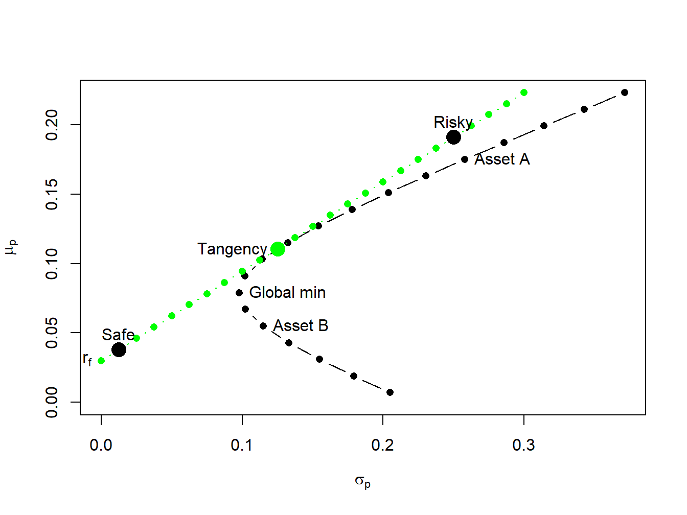
Figure 11.9: The efficient portfolio labeled “safe” has 10% invested in the tangency portfolio and 90% invested in T-Bills; the efficient portfolio labeled “risky” has 200% invested in the tangency portfolio and -100% invested in T-Bills.
11.5.3 Interpreting Efficient Portfolios
As we have seen, efficient portfolios are those portfolios that have the highest expected return for a given level of risk as measured by portfolio standard deviation. For portfolios with expected returns above the T-bill rate, efficient portfolios can also be characterized as those portfolios that have minimum risk (as measured by portfolio standard deviation) for a given target expected return.
To illustrate, consider Figure 11.10 which shows the portfolio frontier for two risky assets and the efficient frontier for two risky assets plus T-Bills. Suppose an investor initially holds all of his wealth in asset \(B\). The expected return on this portfolio is \(\mu_{B}=0.055\), and the standard deviation (risk) is \(\sigma_{B}=0.115\). An efficient portfolio (combinations of the tangency portfolio and T-bills) that has the same standard deviation (risk) as asset \(B\) is given by the portfolio on the efficient frontier that is directly above \(\sigma_{B}=0.115\). To find the shares in the tangency portfolio and T-bills in this portfolio recall from (11.18) that the standard deviation of an efficient portfolio with \(x_{T}\) invested in the tangency portfolio and \(1-x_{T}\) invested in T-bills is \(\sigma_{p}^{e}=x_{T}\sigma_{tan}\). Since we want to find the efficient portfolio with \(\sigma_{p}^{e}=\sigma_{B}=0.115\), we solve: \[ x_{T}=\frac{\sigma_{B}}{\sigma_{tan}}=\frac{0.115}{0.1251}=0.9195,~x_{f}=1-x_{T}=0.08049. \] That is, if we invest \(91.95\%\) of our wealth in the tangency portfolio and \(8.049\%\) in T-bills we will have a portfolio with the same standard deviation as asset B. Since this is an efficient portfolio, the expected return should be higher than the expected return on asset B. Indeed it is since: \[ \mu_{p}^{e}=r_{f}+x_{T}(\mu_{tan}-r_{f})=0.03+0.9195(0.1105-0.03)=0.1040. \] Notice that by diversifying our holding into assets \(A\), \(B\) and T-bills we can obtain a portfolio with the same risk as asset B but with almost twice the expected return! By moving from asset B into an efficient portfolio we raise the Sharpe ratio of the investment from \(SR_{B}=0.217\) to \(SR_{tan}=0.6434\).
Next, consider finding an efficient portfolio that has the same expected return as asset \(B\). Visually, this involves finding the combination of the tangency portfolio and T-bills that corresponds with the intersection of a horizontal line with intercept \(\mu_{B}=0.055\) and the line representing efficient combinations of T-bills and the tangency portfolio. To find the shares in the tangency portfolio and T-bills in this portfolio recall from (11.17) that the expected return of an efficient portfolio with \(x_{T}\) invested in the tangency portfolio and \(1-x_{T}\) invested in T-bills has expected return equal to \(\mu_{p}^{e}=r_{f}+x_{T}(\mu_{tan}-r_{f})\). Since we want to find the efficient portfolio with \(\mu_{p}^{e}=\mu_{B}=0.055\) we solve: \[ x_{T}=\frac{\mu_{p}^{e}-r_{f}}{\mu_{tan}-r_{f}}=\frac{0.055-0.03}{0.1105-0.03}=0.3105,~x_{f}=1-x_{T}=0.6895. \] That is, if we invest \(31.05\%\) of wealth in the tangency portfolio and \(68.95\%\) of our wealth in T-bills we have a portfolio with the same expected return as asset B. Since this is an efficient portfolio, the standard deviation (risk) of this portfolio should be lower than the standard deviation on asset \(B\). Indeed it is since: \[ \sigma_{p}^{e}=x_{T}\sigma_{tan}=0.3105(0.124)=0.03884. \] Notice how large the risk reduction is by forming an efficient portfolio. The standard deviation on the efficient portfolio is almost three times smaller than the standard deviation of asset \(B\)! Again, by moving from asset B into an efficient portfolio we raise the Sharpe ratio of the investment from \(SR_{B}=0.217\) to \(SR_{tan}=0.6434\)
\(\blacksquare\)
The above example illustrates two ways to interpret the benefits from forming efficient portfolios. Starting from some benchmark portfolio, we can fix standard deviation (risk) at the value for the benchmark and then determine the gain in expected return from forming a diversified portfolio72. The gain in expected return has concrete meaning. Alternatively, we can fix expected return at the value for the benchmark and then determine the reduction in standard deviation (risk) from forming a diversified portfolio. The meaning to an investor of the reduction in standard deviation is not as clear as the meaning to an investor of the increase in expected return. It would be helpful if the risk reduction benefit can be translated into a number that is more interpretable than the standard deviation. The concept of Value-at-Risk (VaR) provides such a translation.
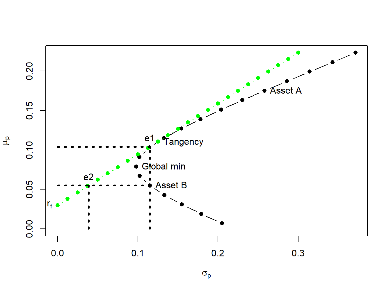
Figure 11.10: The point “e1” represents an efficient portfolio with the same standard deviation as asset \(B\); the point “e2” represents an efficient portfolio with the same expected returns as asset \(B\).
11.5.4 Efficient Portfolios and Value-at-Risk
Recall, the VaR of an investment is the (lower bound of) loss in investment value over a given horizon with a stated probability. For example, consider an investor who invests \(W_{0}=\) \(\$100,000\) in asset \(B\) over the next year. Assuming that \(R_{B}\sim N(0.055,(0.115)^{2})\) represents the annual simple return on asset \(B\), the 5% VaR is: \[ \mathrm{VaR}_{B,0.05}=-q_{0.05}^{R_{B}}W_{0}=(0.055+0.115(-1.645))\cdot\$100,000=\$13,416. \] If an investor holds $100,000 in asset B over the next year, then there is a 5% probability that he will lose $13,416 or more.
Now suppose the investor chooses to hold an efficient portfolio with the same expected return as asset \(B\). This portfolio consists of \(31.05\%\) in the tangency portfolio and \(68.95\%\) in T-bills and has a standard deviation equal to \(0.03884\). Then \(R_{p}\sim N(0.055,0.03884)\) and the 5% VaR on the portfolio is: \[ \mathrm{VaR}_{p,0.05}=-q_{0.05}^{R_{p}}W_{0}=(0.055+0.03884(-1.645))\cdot\$100,000=\$884. \] Notice that the 5% VaR for the efficient portfolio is almost fifteen times smaller than the 5% VaR for the investment in asset \(B\). Since VaR translates risk into a dollar figure, it is more interpretable than standard deviation as a measure of investment risk.
The gain in expected return by investing in an efficient portfolio abstracts from the costs associated with selling the benchmark portfolio and buying the efficient portfolio.↩︎