12.7 Portfolio Analysis Functions in R
The package IntroCompFinR contains a few R functions for computing Markowitz mean-variance efficient portfolios allowing for short sales using matrix algebra computations. These functions allow for the easy computation of the global minimum variance portfolio, an efficient portfolio with a given target expected return, the tangency portfolio, and the efficient frontier. These functions are summarized in Table 12.2.
| Function | Description |
|---|---|
getPortfolio |
create portfolio object |
globalMin.portfolio |
compute global minimum variance portfolio |
efficient.portfolio |
compute minimum variance portfolio subject to target return |
tangency.portfolio |
compute tangency portfolio |
efficient.frontier |
compute efficient frontier of risky assets |
The following examples illustrate the use of the functions in Table 12.2 using the example data in Table 12.1:
##   MSFT   NORD   SBUX
## 0.0427 0.0015 0.0285## MSFT NORD SBUX
## MSFT 0.0100 0.0018 0.0011
## NORD 0.0018 0.0109 0.0026
## SBUX 0.0011 0.0026 0.0199## [1] 0.005To specify a portfolio object, you need an expected
return vector and covariance matrix for the assets under consideration
as well as a vector of portfolio weights. To create an equally weighted
portfolio use:
library(IntroCompFinR)
ew = rep(1,3)/3
equalWeight.portfolio = getPortfolio(er=mu.vec,cov.mat=sigma.mat,weights=ew)
class(equalWeight.portfolio)
## [1] "portfolio"Portfolio objects have the following components:
## [1] "call" "er" "sd" "weights"There are print(), summary() and plot()
methods for portfolio objects. The print() method gives:
## Call:
## getPortfolio(er = mu.vec, cov.mat = sigma.mat, weights = ew)
##
## Portfolio expected return:     0.0242
## Portfolio standard deviation:  0.0759
## Portfolio weights:
##  MSFT  NORD  SBUX
## 0.333 0.333 0.333
The plot() method shows a bar chart of the portfolio weights:
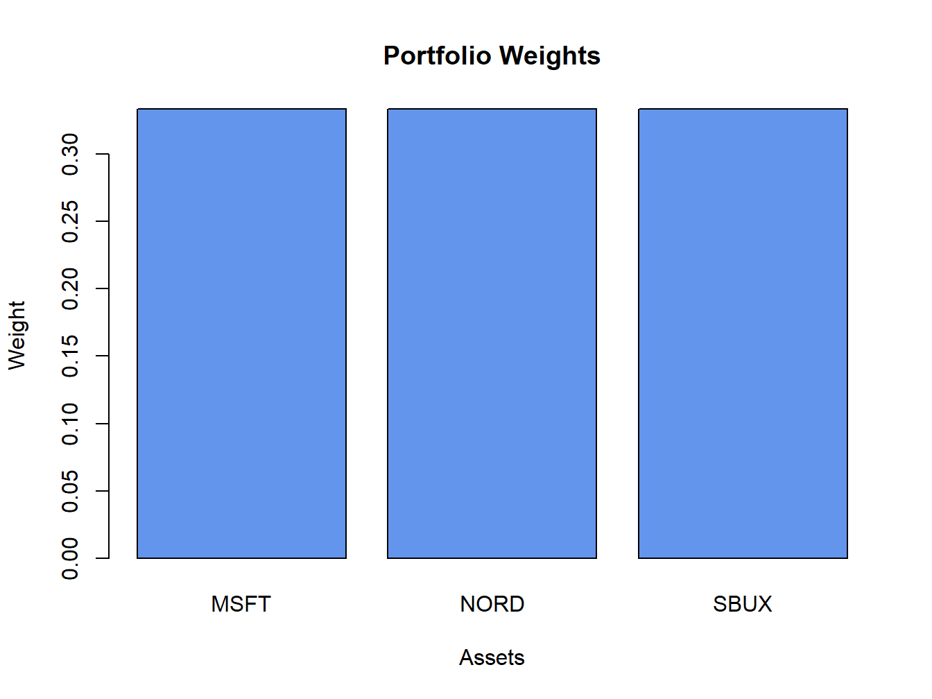
Figure 12.11: Plot method for objects of class “portfolio”
The resulting plot is shown in Figure 12.11.
The global minimum variance portfolio (allowing for short sales) \(\mathbf{m}\)
solves the optimization problem (12.2)
and is computed using (12.6). To
compute this portfolio use the function globalMin.portfolio():
## [1] "portfolio"## Call:
## globalMin.portfolio(er = mu.vec, cov.mat = sigma.mat)
##
## Portfolio expected return: 0.0249
## Portfolio standard deviation: 0.0727
## Portfolio weights:
## MSFT NORD SBUX
## 0.441 0.366 0.193A mean-variance efficient portfolio \(\mathbf{x}\) that achieves the
target expected return \(\mu_{0}\) solves the optimization problem
(12.10) and is computed using (12.14).
To compute this portfolio for the target expected return \(\mu_{0}=E[R_{\textrm{msft}}]=0.0427\)
use the efficient.portfolio() function:
target.return = mu.vec[1]
e.port.msft = efficient.portfolio(mu.vec, sigma.mat, target.return)
class(e.port.msft)
## [1] "portfolio"## Call:
## efficient.portfolio(er = mu.vec, cov.mat = sigma.mat, target.return = target.return)
##
## Portfolio expected return: 0.0427
## Portfolio standard deviation: 0.0917
## Portfolio weights:
## MSFT NORD SBUX
## 0.8275 -0.0907 0.2633The tangency portfolio \(\mathbf{t}\) is the portfolio of risky assets
with the highest Sharpe’s slope and has solutions given by (12.26).
To compute this portfolio with \(r_{f}=0.005\) use the tangency.portfolio()
function:
## [1] "portfolio"## Call:
## tangency.portfolio(er = mu.vec, cov.mat = sigma.mat, risk.free = r.f)
##
## Portfolio expected return: 0.0519
## Portfolio standard deviation: 0.112
## Portfolio weights:
## MSFT NORD SBUX
## 1.027 -0.326 0.299The the set of efficient portfolios of risky assets can be computed
as a convex combination of any two efficient portfolios. It is convenient
to use the global minimum variance portfolio as one portfolio and
an efficient portfolio with target expected return equal to the maximum
expected return of the assets under consideration as the other portfolio.
Call these portfolios \(\mathbf{m}\) and \(\mathbf{x}\), respectively.
For any number \(\alpha\), another efficient portfolio can be computed
as:
\[
\mathbf{z}=\alpha\mathbf{x}+(1-\alpha)\mathbf{m}
\]
The function efficient.frontier() constructs the set of efficient
portfolios using this method for a collection of \(\alpha\) values
on an equally spaced grid between \(\alpha_{min}\) and \(\alpha_{max}\).
For example, to compute 20 efficient portfolios for values of \(\alpha\)
between -2 and 1.5 use:
## $names
## [1] "call"    "er"      "sd"      "weights"
##
## $class
## [1] "Markowitz"## Call:
## efficient.frontier(er = mu.vec, cov.mat = sigma.mat, nport = 20,
## alpha.min = -0.5, alpha.max = 2)
##
## Frontier portfolios' expected returns and standard deviations
## port 1 port 2 port 3 port 4 port 5 port 6 port 7 port 8 port 9 port 10
## ER 0.0160 0.0183 0.0207 0.0230 0.0254 0.0277 0.0300 0.0324 0.0347 0.0371
## SD 0.0779 0.0755 0.0739 0.0729 0.0727 0.0732 0.0745 0.0764 0.0790 0.0821
## port 11 port 12 port 13 port 14 port 15 port 16 port 17 port 18 port 19
## ER 0.0394 0.0418 0.0441 0.0464 0.0488 0.0511 0.0535 0.0558 0.0582
## SD 0.0858 0.0899 0.0944 0.0993 0.1044 0.1098 0.1154 0.1212 0.1272
## port 20
## ER 0.0605
## SD 0.1333Use the summary() method to show the weights of these portfolios.
Use the plot() method to create a simple plot the efficient
frontier:
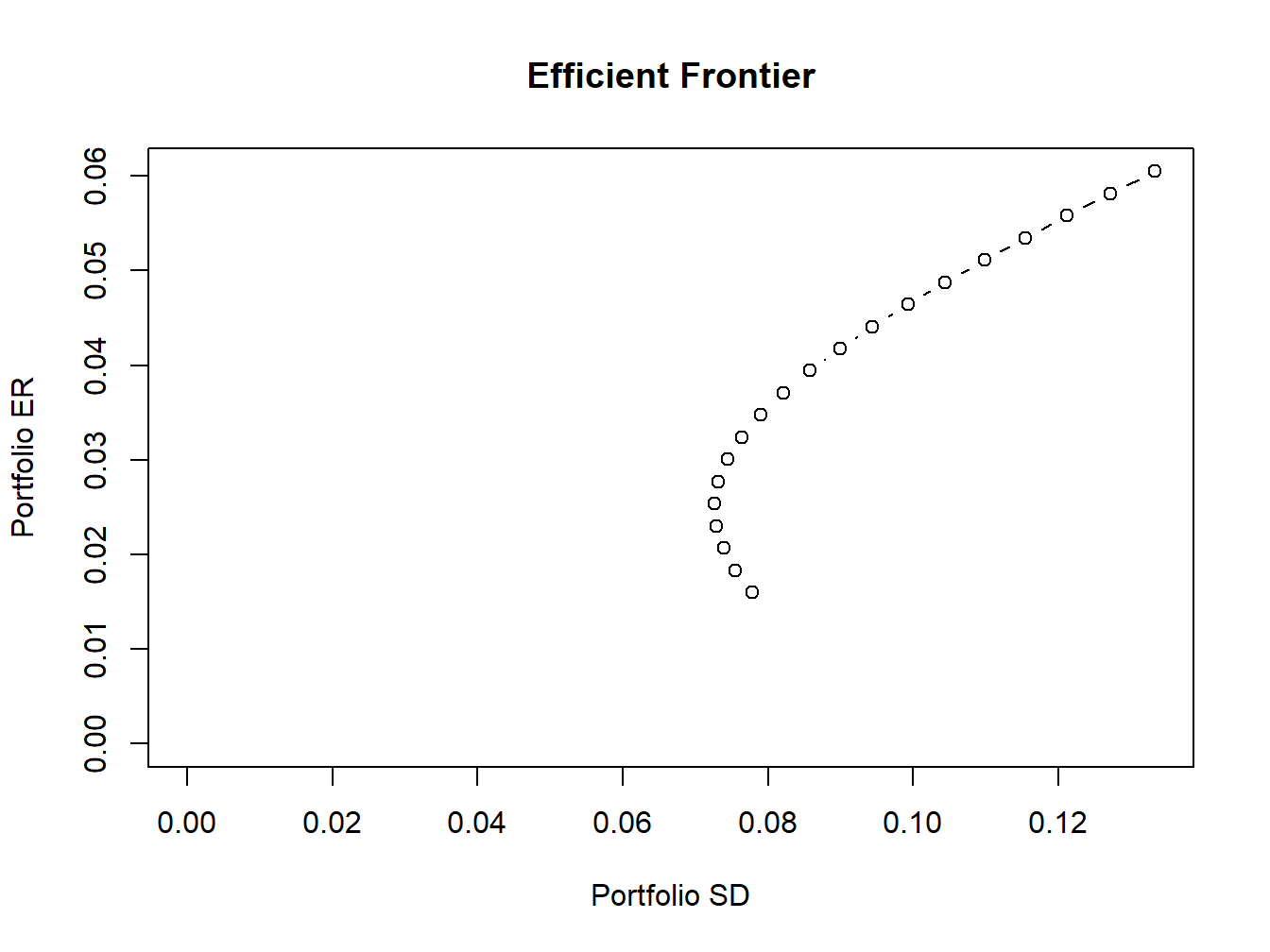
Figure 12.12: Plot method for objects of class “Markowitz”
The resulting plot is shown in Figure 12.12. To create a more elaborate plot of the efficient frontier showing the original assets and the tangency portfolio use:
plot(ef, plot.assets=T, col="blue", pch=16)
points(gmin.port$sd, gmin.port$er, col="green", pch=16, cex=2)
text(gmin.port$sd, gmin.port$er, labels = "Global min", pos = 4)
points(tan.port$sd, tan.port$er, col="red", pch=16, cex=2)
text(tan.port$sd, tan.port$er, labels = "Tangency", pos = 3)
sr.tan = (tan.port$er - r.f)/tan.port$sd
abline(a=r.f, b=sr.tan, col="green", lwd=2)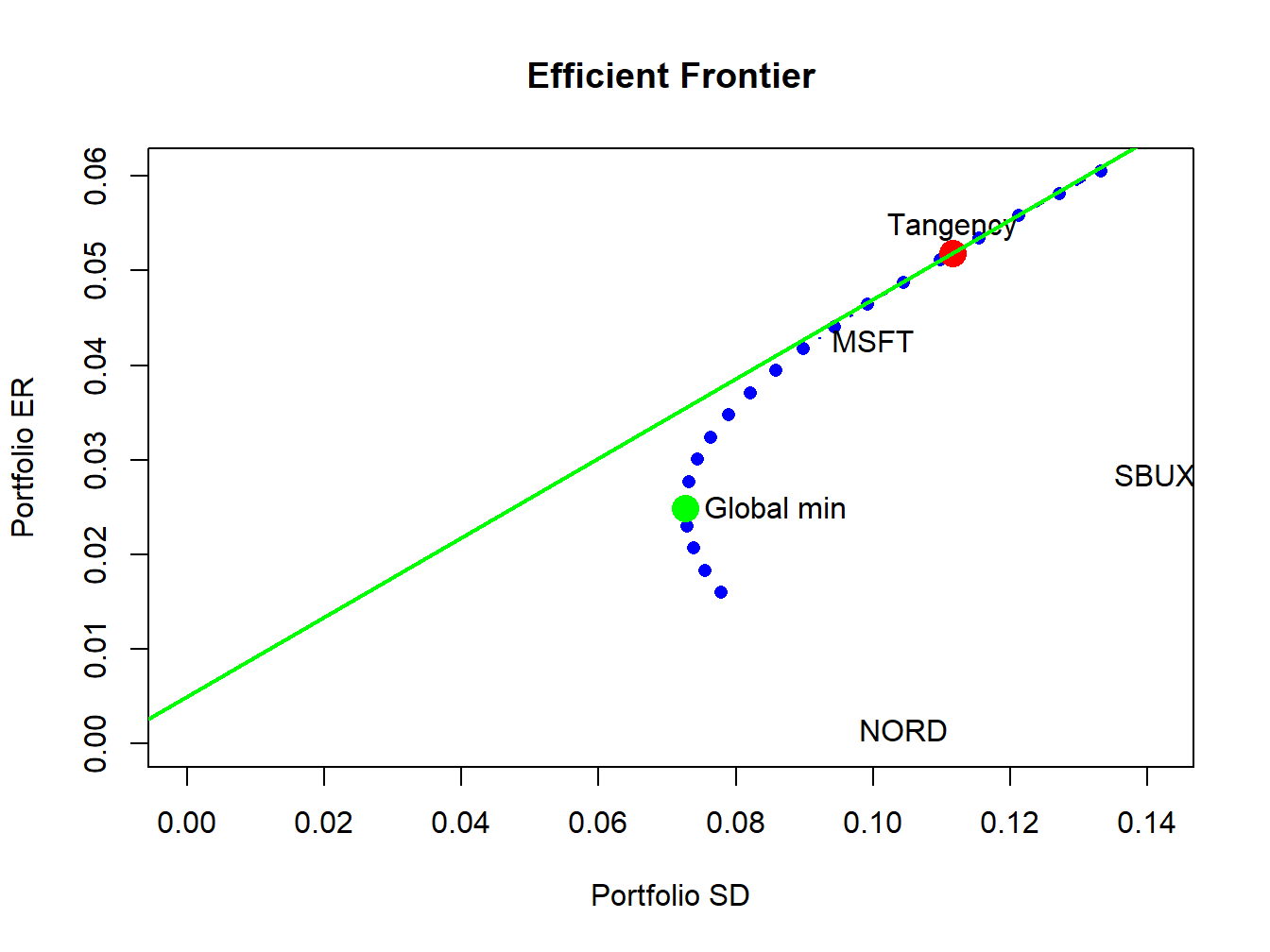
Figure 12.13: Efficient frontier plot.
The resulting plot is shown in Figure 12.13.