12.2 Determining the Global Minimum Variance Portfolio Using Matrix Algebra
The global minimum variance portfolio \(\mathbf{m}=(m_{1},\ldots,m_{N})^{\prime}\) for the \(N\) asset case solves the constrained minimization problem: \[\begin{align} \min_{\mathbf{m}}~\sigma_{p,m}^{2}=\mathbf{m^{\prime}\Sigma m}\,s.t.\,\mathbf{m^{\prime}1}=1.\tag{12.2} \end{align}\] The Lagrangian for this problem is: \[\begin{align*} L(\mathbf{m},\lambda) & =\mathbf{m^{\prime}\Sigma m}+\lambda(\mathbf{m^{\prime}1}-1), \end{align*}\] and the first order conditions (FOCs) for a minimum are: \[\begin{align} \mathbf{0} & =\frac{\partial L}{\partial\mathbf{m}}=\frac{\partial\mathbf{m^{\prime}\Sigma m}}{\partial\mathbf{m}}+\frac{\partial\lambda(\mathbf{m^{\prime}1}-1)}{\partial\mathbf{m}}=2\Sigma \mathbf{m}+\lambda\mathbf{1},\tag{12.3}\\ 0 & =\frac{\partial L}{\partial\lambda}=\frac{\partial\mathbf{m^{\prime}\Sigma m}}{\partial\lambda}+\frac{\partial\lambda(\mathbf{m^{\prime}1}-1)}{\partial\lambda}=\mathbf{m^{\prime}1}-1.\tag{12.4} \end{align}\] The FOCs (12.3)-(12.4) give \(N+1\) linear equations in \(N+1\) unknowns which can be solved to find the global minimum variance portfolio weight vector \(\mathbf{m}\) as follows. The \(N+1\) linear equations describing the first order conditions have the matrix representation: \[\begin{equation} \left(\begin{array}{cc} 2\Sigma & \mathbf{1}\\ \mathbf{1}^{\prime} & 0 \end{array}\right)\left(\begin{array}{c} \mathbf{m}\\ \lambda \end{array}\right)=\left(\begin{array}{c} \mathbf{0}\\ 1 \end{array}\right).\tag{12.5} \end{equation}\] The system (12.5) is of the form \(\mathbf{A}_{m}\mathbf{z}_{m}=\mathbf{b}\), where: \[ \mathbf{A}_{m}=\left(\begin{array}{cc} 2\Sigma & \mathbf{1}\\ \mathbf{1}^{\prime} & 0 \end{array}\right),~\mathbf{z}_{m}=\left(\begin{array}{c} \mathbf{m}\\ \lambda \end{array}\right)\textrm{ and }\mathbf{b}=\left(\begin{array}{c} \mathbf{0}\\ 1 \end{array}\right). \] Provided \(\mathbf{A}_{m}\) is invertible, the solution for \(\mathbf{z}_{m}\) is:79 \[\begin{equation} \mathbf{z}_{m}=\mathbf{A}_{m}^{-1}\mathbf{b}.\tag{12.6} \end{equation}\] The first \(N\) elements of \(\mathbf{z}_{m}\) is the portfolio weight vector \(\mathbf{m}\) for the global minimum variance portfolio with expected return \(\mu_{p,m}=\mathbf{m}^{\prime}\mu\) and variance \(\sigma_{p,m}^{2}=\mathbf{m}^{\prime}\Sigma \mathbf{m}\).
Using the data in Table 12.1, we can use R to compute the global minimum variance portfolio weights from (12.6) as follows:
top.mat = cbind(2*sigma.mat, rep(1, 3))
bot.vec = c(rep(1, 3), 0)
Am.mat = rbind(top.mat, bot.vec)
b.vec = c(rep(0, 3), 1)
z.m.mat = solve(Am.mat)%*%b.vec
m.vec = z.m.mat[1:3,1]
m.vec
## MSFT NORD SBUX
## 0.441 0.366 0.193Hence, the global minimum variance portfolio has portfolio weights \(m_{\textrm{msft}}=0.441\), \(m_{\textrm{nord}}=0.366\) and \(m_{\textrm{sbux}}=0.193\), and is given by the vector \(\mathbf{m}=(0.441,0.366,0.193)^{\prime}\). The expected return on this portfolio, \(\mu_{p,m}=\mathbf{m}^{\prime}\mu\), is:
## [1] 0.0249The portfolio variance, \(\sigma_{p,m}^{2}=\mathbf{m}^{\prime}\Sigma \mathbf{m}\), and standard deviation, \(\sigma_{p,m}\), are:
sig2.gmin = as.numeric(t(m.vec)%*%sigma.mat%*%m.vec)
sig.gmin = sqrt(sig2.gmin)
c(sig2.gmin, sig.gmin)
## [1] 0.00528 0.07268In Figure 12.4, this portfolio is labeled “GMIN” .
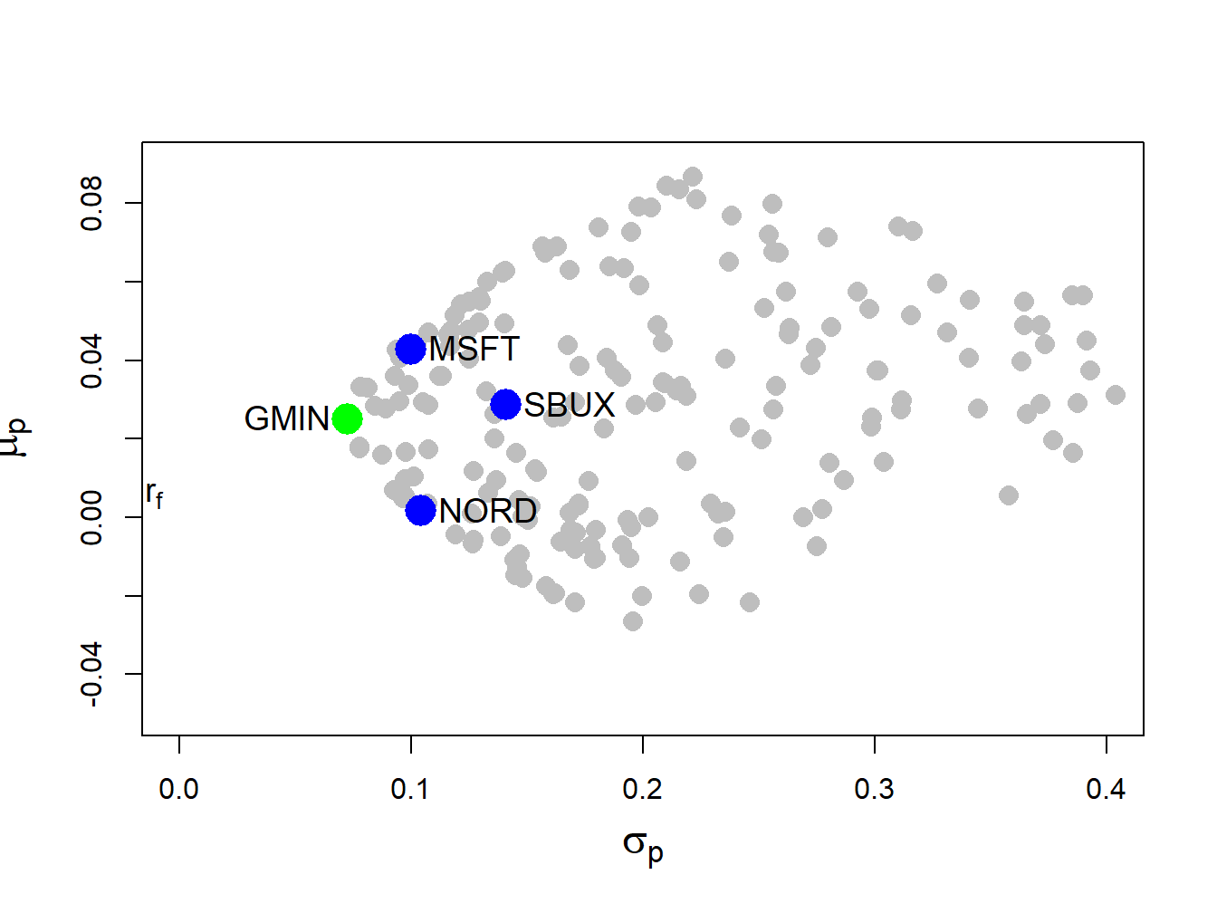
Figure 12.4: Global minimum variance portfolio from example data.
\(\blacksquare\)
12.2.1 Alternative derivation of global minimum variance portfolio
We can use the first order conditions (12.3) - (12.4) to give an explicit solution for the global minimum variance portfolio \(\mathbf{m}\) as follows. First, use (12.3) to solve for \(\mathbf{m}\) as a function of \(\lambda\): \[\begin{equation} \mathbf{m}=-\frac{1}{2}\cdot\lambda\Sigma^{-1}\mathbf{1}.\tag{12.7} \end{equation}\] Next, multiply both sides of (12.7) by \(\mathbf{1}^{\prime}\) and use (12.4) to solve for \(\lambda\): \[\begin{align*} 1 & =\mathbf{1}^{\prime}\mathbf{m}=-\frac{1}{2}\cdot\lambda\mathbf{1}^{\prime}\Sigma^{-1}\mathbf{1}\\ & \Rightarrow\lambda=-2\cdot\frac{1}{\mathbf{1}^{\prime}\Sigma^{-1}\mathbf{1}}. \end{align*}\] Finally, substitute the value for \(\lambda\) back into (12.7) to solve for \(\mathbf{m}\): \[\begin{equation} \mathbf{m}=-\frac{1}{2}\left(-2\right)\frac{1}{\mathbf{1}^{\prime}\Sigma^{-1}\mathbf{1}}\Sigma^{-1}\mathbf{1}=\frac{\Sigma^{-1}\mathbf{1}}{\mathbf{1}^{\prime}\Sigma^{-1}\mathbf{1}}.\tag{12.8} \end{equation}\] Notice that (12.8) shows that a solution for \(\mathbf{m}\) exists as long as \(\Sigma\) is invertible.
Using the data in Table 12.1, we can use R to compute the global minimum variance portfolio weights from (12.8) as follows:
one.vec = rep(1, 3)
sigma.inv.mat = solve(sigma.mat)
top.mat = sigma.inv.mat%*%one.vec
bot.val = as.numeric((t(one.vec)%*%sigma.inv.mat%*%one.vec))
m.mat = top.mat/bot.val
m.mat[,1]
## MSFT NORD SBUX
## 0.441 0.366 0.193\(\blacksquare\)
For \(\mathbf{A}_{m}\) to be invertible we need \(\Sigma\) to be invertible, which requires \(|\rho_{ij}|\neq1\) for \(i\neq j\) and \(\sigma_{i}^{2}>0\) for all \(i\).↩︎