2.2 Bivariate Distributions

So far we have only considered probability distributions for a single random variable. In many situations, we want to be able to characterize the probabilistic behavior of two or more random variables simultaneously. For example, we might want to know about the probabilistic behavior of the returns on a two asset portfolio. In this section, we discuss bivariate distributions and important concepts related to the analysis of two random variables.

2.2.1 Discrete random variables

Let \(X\) and \(Y\) be discrete random variables with sample spaces \(S_{X}\) and \(S_{Y}\), respectively. The likelihood that \(X\) and \(Y\) takes values in the joint sample space \(S_{XY}=S_{X}\times S_{Y}\) (Cartesian product of the individual sample spaces) is determined by the joint probability distribution \(p(x,y)=\Pr(X=x,Y=y).\) The function \(p(x,y)\) satisfies:

• 1. \(p(x,y)>0\) for \(x,y\in S_{XY}\);
• 2. \(p(x,y)=0\) for \(x,y\notin S_{XY}\);
• 3. \(\sum_{x,y\in S_{XY}}p(x,y)=\sum_{x\in S_{X}}\sum_{y\in S_{Y}}p(x,y)=1\).

Example 2.39 (Bivariate discrete distribution for stock returns)

Let \(X\) denote the monthly return (in percent) on Microsoft stock and let \(Y\) denote the monthly return on Starbucks stock. For simplicity suppose that the sample spaces for \(X\) and \(Y\) are \(S_{X}=\{0,1,2,3\}\) and \(S_{Y}=\{0,1\}\) so that the random variables \(X\) and \(Y\) are discrete. The joint sample space is the two dimensional grid \(S_{XY}=\{(0,0)\), \((0,1)\), \((1,0)\), \((1,1)\), \((2,0)\), \((2,1)\), \((3,0)\), \((3,1)\}\). Table 2.3 illustrates the joint distribution for \(X\) and \(Y\). From the table, \(p(0,0)=\Pr(X=0,Y=0)=1/8\). Notice that the sum of all the entries in the table sum to unity.

\(\blacksquare\)

+——+————–+———+———+————–+ | | |Y | | | +======+==============+=========+=========+==============+ | |% |0 |1 |\(\Pr(X)\) | +——+————–+———+———+————–+ | |0 |1/8 |0 |1/8 | +——+————–+———+———+————–+ |X |1 |2/8 |1/8 |3/8 | +——+————–+———+———+————–+ | |2 |1/8 |2/8 |3/8 | +——+————–+———+———+————–+ | |3 |0 |1/8 |1/8 | +——+————–+———+———+————–+ | |\(\Pr(Y)\) |4/8 |4/8 |1 | +——+————–+———+———+————–+ Table: (#tab:Table-bivariateDistn) Discrete bivariate distribution for Microsoft and Starbucks stock prices.

2.2.1.1 Marginal Distributions

The joint probability distribution tells us the probability of \(X\) and \(Y\) occurring together. What if we only want to know about the probability of \(X\) occurring, or the probability of \(Y\) occurring?

Example 2.40 (Find \(\Pr(X=0)\) and \(\Pr(Y=1)\) from joint distribution)

Consider the joint distribution in Table 2.3. What is \(\Pr(X=0)\) regardless of the value of \(Y\)? Now \(X\) can occur if \(Y=0\) or if \(Y=1\) and since these two events are mutually exclusive we have that \[ \Pr(X=0)=\Pr(X=0,Y=0)+\Pr(X=0,Y=1)=0+1/8=1/8. \] Notice that this probability is equal to the horizontal (row) sum of the probabilities in the table at \(X=0\). We can find \(\Pr(Y=1)\) in a similar fashion: \[\begin{align*} \Pr(Y=1)&=\Pr(X=0,Y=1)+\Pr(X=1,Y=1)+\Pr(X=2,Y=1)+\Pr(X=3,Y=1)\\ &=0+1/8+2/8+1/8=4/8. \end{align*}\] This probability is the vertical (column) sum of the probabilities in the table at \(Y=1\).

\(\blacksquare\)

Definition 2.15 The probability \(\Pr(X=x)\) is called the marginal probability of \(X\) and is given by: \[\begin{equation} \Pr(X=x)=\sum_{y\in S_{Y}}\Pr(X=x,Y=y).\tag{2.26} \end{equation}\] Similarly, the marginal probability of \(Y=y\) is given by: \[\begin{equation} \Pr(Y=y)=\sum_{x\in S_{X}}\Pr(X=x,Y=y).\tag{2.27} \end{equation}\]

Example 2.41 (Marginal probabilities of discrete bivariate distribution)

The marginal probabilities of \(X=x\) are given in the last column of Table 2.3, and the marginal probabilities of \(Y=y\) are given in the last row of Table 2.3. Notice that these probabilities sum to 1. For future reference we note that \(E[X]=3/2,\mathrm{var}(X)=3/4,E[Y]=1/2\), and \(\mathrm{var}(Y)=1/4\).

\(\blacksquare\)

2.2.1.2 Conditional Distributions

For random variables in Table 2.3, suppose we know that the random variable \(Y\) takes on the value \(Y=0\). How does this knowledge affect the likelihood that \(X\) takes on the values 0, 1, 2 or 3? For example, what is the probability that \(X=0\) given that we know \(Y=0\)? To find this probability, we use Bayes’ law and compute the conditional probability: \[ \Pr(X=0|Y=0)=\frac{\Pr(X=0,Y=0)}{\Pr(Y=0)}=\frac{1/8}{4/8}=1/4. \] The notation \(\Pr(X=0|Y=0)\) is read as “the probability that \(X=0\) given that \(Y=0\)” . Notice that \(\Pr(X=0|Y=0)=1/4>\Pr(X=0)=1/8\). Hence, knowledge that \(Y=0\) increases the likelihood that \(X=0\). Clearly, \(X\) depends on \(Y\).

Now suppose that we know that \(X=0\). How does this knowledge affect the probability that \(Y=0?\) To find out we compute: \[ \Pr(Y=0|X=0)=\frac{\Pr(X=0,Y=0)}{\Pr(X=0)}=\frac{1/8}{1/8}=1. \] Notice that \(\Pr(Y=0|X=0)=1>\Pr(Y=0)=1/2\). That is, knowledge that \(X=0\) makes it certain that \(Y=0\).

Definition 2.16 The conditional probability that \(X=x\) given that \(Y=y\) (provided \(\Pr(Y=y)\neq0)\) is, \[\begin{equation} p(x|y) = \Pr(X=x|Y=y)=\frac{\Pr(X=x,Y=y)}{\Pr(Y=y)} = \frac{p(x,y)}{p(y)},\tag{2.28} \end{equation}\] and the conditional probability that \(Y=y\) given that \(X=x\) (provided \(\Pr(X=x)\neq0\)) is, \[\begin{equation} p(y|x) = \Pr(Y=y|X=x)=\frac{\Pr(X=x,Y=y)}{\Pr(X=x)} = \frac{p(x,y)}{p(x)}.\tag{2.29} \end{equation}\]

Example 2.42 (Conditional distributions)

For the bivariate distribution in Table 2.3, the conditional probabilities along with marginal probabilities are summarized in Tables 2.4 and 2.5. Notice that the marginal distribution of \(X\) is centered at \(x=3/2\) whereas the conditional distribution of \(X|Y=0\) is centered at \(x=1\) and the conditional distribution of \(X|Y=1\) is centered at \(x=2\).

\(\blacksquare\)

+—+————+————–+————–+ |x |\(\Pr(X=x)\) |\(\Pr(X|Y=0)\) |\(\Pr(X|Y=1)\) | +===+============+==============+==============+ |0 |1/8 |2/8 |0 | +—+————+————–+————–+ |1 |3/8 |4/8 |2/8 | +—+————+————–+————–+ |2 |3/8 |4/8 |4/8 | +—+————+————–+————–+ |3 |1/8 |0 |2/8 | +—+————+————–+————–+ Table: (#tab:Table-ConditionalDistnX) Conditional probability distribution of X from bivariate discrete distribution.

+—+————+————–+————–+————–+————–+ |y |\(\Pr(Y=y)\) |\(\Pr(Y|X=0)\) |\(\Pr(Y|X=1)\) |\(\Pr(Y|X=2)\) |\(\Pr(Y|X=3)\) | +—+————+————–+————–+————–+————–+ |0 |1/2 |1 |2/3 |1/3 |0 | +—+————+————–+————–+————–+————–+ |1 |1/2 |0 |1/3 |2/3 |1 | +—+————+————–+————–+————–+————–+ Table: (#tab:Table-ConditionalDistnY) Conditional distribution of Y from bivariate discrete distribution.

2.2.1.3 Conditional expectation and conditional variance

Just as we defined shape characteristics of the marginal distributions of \(X\) and \(Y\), we can also define shape characteristics of the conditional distributions of \(X|Y=y\) and \(Y|X=x\). The most important shape characteristics are the conditional expectation (conditional mean) and the conditional variance. The conditional mean of \(X|Y=y\) is denoted by \(\mu_{X|Y=y}=E[X|Y=y]\), and the conditional mean of \(Y|X=x\) is denoted by \(\mu_{Y|X=x}=E[Y|X=x]\).

Definition 2.17 For discrete random variables \(X\) and \(Y\), the conditional expectations are defined as: \[\begin{align} \mu_{X|Y=y} & =E[X|Y=y]=\sum_{x\in S_{X}}x\cdot\Pr(X=x|Y=y),\tag{2.30}\\ \mu_{Y|X=x} & =E[Y|X=x]=\sum_{y\in S_{Y}}y\cdot\Pr(Y=y|X=x).\tag{2.31} \end{align}\]

Similarly, the conditional variance of \(X|Y=y\) is denoted by \(\sigma_{X|Y=y}^{2}=\mathrm{var}(X|Y=y)\) and the conditional variance of \(Y|X=x\) is denoted by \(\sigma_{Y|X=x}^{2}=\mathrm{var}(Y|X=x)\).

Definition 2.18 For discrete random variables \(X\) and \(Y\), the conditional variances are defined as: \[\begin{align} \sigma_{X|Y=y}^{2} & =\mathrm{var}(X|Y=y)=\sum_{x\in S_{X}}(x-\mu_{X|Y=y})^{2}\cdot\Pr(X=x|Y=y),\tag{2.32}\\ \sigma_{Y|X=x}^{2} & =\mathrm{var}(Y|X=x)=\sum_{y\in S_{Y}}(y-\mu_{Y|X=x})^{2}\cdot\Pr(Y=y|X=x).\tag{2.33} \end{align}\] The conditional volatilities are defined as: \[\begin{align} \sigma_{X|Y=y} & = \sqrt{\sigma_{X|Y=y}^{2}}, \tag{2.34}\\ \sigma_{Y|X=x} & = \sqrt{\sigma_{Y|X=x}^{2}}. \tag{2.35} \end{align}\]

Then conditional mean is the center of mass of the conditional distribution, and the conditional variance and volatility measure the spread of the conditional distribution about the conditional mean.

Example 2.43 (Compute conditional expectation and conditional variance)

For the random variables in Table 2.3, we have the following conditional moments for \(X\): \[\begin{align*} E[X|Y & =0]=0\cdot1/4+1\cdot1/2+2\cdot1/4+3\cdot0=1,\\ E[X|Y & =1]=0\cdot0+1\cdot1/4+2\cdot1/2+3\cdot1/4=2,\\ \mathrm{var}(X|Y & =0)=(0-1)^{2}\cdot1/4+(1-1)^{2}\cdot1/2+(2-1)^{2}\cdot1/2+(3-1)^{2}\cdot0=1/2,\\ \mathrm{var}(X|Y & =1)=(0-2)^{2}\cdot0+(1-2)^{2}\cdot1/4+(2-2)^{2}\cdot1/2+(3-2)^{2}\cdot1/4=1/2. \end{align*}\] Compare these values to \(E[X]=3/2\) and \(\mathrm{var}(X)=3/4\). Notice that \(\mathrm{var}(X|Y) = 1/2 < \mathrm{var}(X)=3/4\) so that conditioning on information reduces variability. Also, notice that as \(y\) increases, \(E[X|Y=y]\) increases.

For \(Y\), similar calculations gives: \[\begin{align*} E[Y|X & =0]=0,E[Y|X=1]=1/3,E[Y|X=2]=2/3,E[Y|X=3]=1,\\ \mathrm{var}(Y|X & =0)=0,\mathrm{var}(Y|X=1)=0.2222,\mathrm{var}(Y|X=2)=0.2222,\mathrm{var}(Y|X=3)=0. \end{align*}\] Compare these values to \(E[Y]=1/2\) and \(\mathrm{var}(Y)=1/4\). Notice that as \(x\) increases \(E[Y|X=x]\) increases.

\(\blacksquare\)

2.2.1.4 Conditional expectation and the regression function

Consider the problem of predicting the value \(Y\) given that we know \(X=x\). A natural predictor to use is the conditional expectation \(E[Y|X=x]\). In this prediction context, the conditional expectation \(E[Y|X=x]\) is called the regression function. The graph with \(E[Y|X=x]\) on the vertical axis and \(x\) on the horizontal axis gives the regression line. The relationship between \(Y\) and the regression function may be expressed using the trivial identity: \[\begin{align} Y & =E[Y|X=x]+Y-E[Y|X=x]\nonumber \\ & =E[Y|X=x]+\varepsilon,\tag{2.36} \end{align}\] where \(\varepsilon=Y-E[Y|X]\) is called the regression error.

Example 2.44 (Regression line for bivariate discrete distribution)

For the random variables in Table 2.3, the regression line is plotted in Figure 2.11. Notice that there is a linear relationship between \(E[Y|X=x]\) and \(x\). When such a linear relationship exists we call the regression function a linear regression. Linearity of the regression function, however, is not guaranteed. It may be the case that there is a non-linear (e.g., quadratic) relationship between \(E[Y|X=x]\) and \(x\). In this case, we call the regression function a non-linear regression.

\(\blacksquare\)

Figure 2.11: Regression function \(E[Y|X=x]\) from discrete bivariate distribution.

2.2.1.5 Law of Total Expectations

Before \(Y\) is observed, \(E[X|Y]\) is a random variable because its value depends on the value of \(Y\) which is a random variable. Similarly, \(E[Y|X]\) is also a random variable. Since \(E[X|Y]\) and \(E[Y|X]\) are random variables we can consider their mean values. To illustrate, for the random variables in Table 2.3 notice that: \[\begin{align*} E[X] & = sum_{y \in S_{Y}} E[X|Y=y]\cdot \Pr(Y=y)\\ & =E[X|Y=0]\cdot\Pr(Y=0)+E[X|Y=1]\cdot\Pr(Y=1)\\ & =1\cdot1/2+2\cdot1/2=3/2, \end{align*}\] and, \[\begin{align*} E[Y] & = sum_{x \in S_{X}} E[Y|X=x]\cdot \Pr(X=x)\\ & =E[Y|X=0]\cdot\Pr(X=0)+E[Y|X=1]\cdot\Pr(X=1)\\ +E[Y|X & =2]\cdot\Pr(X=2)+E[Y|X=3]\cdot\Pr(X=3)=1/2. \end{align*}\] This result is known as the law of total expectations.

Proposition 2.2 For two random variables \(X\) and \(Y\) (discrete or continuous) we have, \[\begin{align} E[X] & =E[E[X|Y]],\tag{2.37}\\ E[Y] & =E[E[Y|X]],\nonumber \end{align}\] where the expectation on the first line is taken with respect to the random variable \(Y\), and the the expectation on the second line is taken with respect to the random variable \(X\).

In words, the law of total expectations says that the mean of the conditional mean is the unconditional mean.

2.2.2 Bivariate distributions for continuous random variables

Let \(X\) and \(Y\) be continuous random variables defined over the real line. We characterize the joint probability distribution of \(X\) and \(Y\) using the joint probability function (pdf) \(f(x,y)\) such that \(f(x,y)\geq0\) and, \[ \int_{-\infty}^{\infty}\int_{-\infty}^{\infty}f(x,y)~dx~dy=1. \] The three-dimensional plot of the joint probability distribution gives a probability surface whose total volume is unity. To compute joint probabilities of \(x_{1}\leq X\leq x_{2}\) and \(y_{1}\leq Y\leq y_{2},\) we need to find the volume under the probability surface over the grid where the intervals \([x_{1},x_{2}]\) and \([y_{1},y_{2}]\) overlap. Finding this volume requries solving the double integral: \[ \Pr(x_{1}\leq X\leq x_{2},y_{1}\leq Y\leq y_{2})=\int_{x_{1}}^{x_{2}}\int_{y_{1}}^{y_{2}}f(x,y)~dx~dy. \]

Example 2.45 (Standard bivariate normal distribution)

A standard bivariate normal pdf for \(X\) and \(Y\) has the form: \[\begin{equation} f(x,y)=\frac{1}{2\pi}e^{-\frac{1}{2}(x^{2}+y^{2})},~-\infty\leq x,~y\leq\infty\tag{2.38} \end{equation}\] and has the shape of a symmetric bell (think Liberty Bell) centered at \(x=0\) and \(y=0\). To find \(\Pr(-1<X<1,-1<Y<1)\) we must solve: \[ \int_{-1}^{1}\int_{-1}^{1}\frac{1}{2\pi}e^{-\frac{1}{2}(x^{2}+y^{2})}~dx~dy, \] which, unfortunately, does not have an analytical solution. Numerical approximation methods are required to evaluate the above integral. The function pmvnorm() in the R package mvtnorm can be used to evaluate areas under the bivariate standard normal surface. To compute \(\Pr(-1<X<1,-1<Y<1)\) use:

library(mvtnorm)
pmvnorm(lower=c(-1, -1), upper=c(1, 1))

## [1] 0.4660649
## attr(,"error")
## [1] 1e-15
## attr(,"msg")
## [1] "Normal Completion"

Here, \(\Pr(-1<X<1,-1<Y<1)=0.4661\). The attribute error gives the estimated absolute error of the approximation, and the attribute message tells the status of the algorithm used for the approximation. See the online help for pmvnorm for more details.

\(\blacksquare\)

2.2.2.1 Marginal and conditional distributions

The marginal pdf of \(X\) is found by integrating \(y\) out of the joint pdf \(f(x,y)\) and the marginal pdf of \(Y\) is found by integrating \(x\) out of the joint pdf \(f(x,y)\): \[\begin{align} f(x) & =\int_{-\infty}^{\infty}f(x,y)~dy,\tag{2.39}\\ f(y) & =\int_{-\infty}^{\infty}f(x,y)~dx.\tag{2.40} \end{align}\] The conditional pdf of \(X\) given that \(Y=y\), denoted \(f(x|y)\), is computed as \[\begin{equation} f(x|y)=\frac{f(x,y)}{f(y)},\tag{2.41} \end{equation}\] and the conditional pdf of \(Y\) given that \(X=x\) is computed as, \[\begin{equation} f(y|x)=\frac{f(x,y)}{f(x)}.\tag{2.42} \end{equation}\] The conditional means are computed as \[\begin{align} \mu_{X|Y=y} & =E[X|Y=y]=\int x\cdot p(x|y)~dx,\tag{2.43}\\ \mu_{Y|X=x} & =E[Y|X=x]=\int y\cdot p(y|x)~dy,\tag{2.44} \end{align}\] and the conditional variances are computed as, \[\begin{align} \sigma_{X|Y=y}^{2} & =\mathrm{var}(X|Y=y)=\int(x-\mu_{X|Y=y})^{2}p(x|y)~dx,\tag{2.45}\\ \sigma_{Y|X=x}^{2} & =\mathrm{var}(Y|X=x)=\int(y-\mu_{Y|X=x})^{2}p(y|x)~dy.\tag{2.46} \end{align}\]

Example 2.46 (Conditional and marginal distributions from bivariate standard normal)

Suppose \(X\) and \(Y\) are distributed bivariate standard normal. To find the marginal distribution of \(X\) we use (2.39) and solve: \[ f(x)=\int_{-\infty}^{\infty}\frac{1}{2\pi}e^{-\frac{1}{2}(x^{2}+y^{2})}~dy=\frac{1}{\sqrt{2\pi}}e^{-\frac{1}{2}x^{2}}\int_{-\infty}^{\infty}\frac{1}{\sqrt{2\pi}}e^{-\frac{1}{2}y^{2}}~dy=\frac{1}{\sqrt{2\pi}}e^{-\frac{1}{2}x^{2}}. \] Hence, the marginal distribution of \(X\) is standard normal. Similiar calculations show that the marginal distribution of \(Y\) is also standard normal. To find the conditional distribution of \(X|Y=y\) we use (2.41) and solve: \[\begin{align*} f(x|y) & =\frac{f(x,y)}{f(x)}=\frac{\frac{1}{2\pi}e^{-\frac{1}{2}(x^{2}+y^{2})}}{\frac{1}{\sqrt{2\pi}}e^{-\frac{1}{2}y^{2}}}\\ & =\frac{1}{\sqrt{2\pi}}e^{-\frac{1}{2}(x^{2}+y^{2})+\frac{1}{2}y^{2}}\\ & =\frac{1}{\sqrt{2\pi}}e^{-\frac{1}{2}x^{2}}\\ & =f(x) \end{align*}\] So, for the standard bivariate normal distribution \(f(x|y)=f(x)\) which does not depend on \(y\). Similar calculations show that \(f(y|x)=f(y)\).

\(\blacksquare\)

2.2.3 Independence

Let \(X\) and \(Y\) be two discrete random variables. Intuitively, \(X\) is independent of \(Y\) if knowledge about \(Y\) does not influence the likelihood that \(X=x\) for all possible values of \(x\in S_{X}\) and \(y\in S_{Y}\). Similarly, \(Y\) is independent of \(X\) if knowledge about \(X\) does not influence the likelihood that \(Y=y\) for all values of \(y\in S_{Y}\). We represent this intuition formally for discrete random variables as follows.

Definition 2.19 Let \(X\) and \(Y\) be discrete random variables with sample spaces \(S_{X}\) and \(S_{Y}\), respectively. \(X\) and \(Y\) are independent random variables if and only if (iff): \[\begin{align*} \Pr(X & =x|Y=y)=\Pr(X=x),\textrm{ for all }x\in S_{X},y\in S_{Y}\\ \Pr(Y & =y|X=x)=\Pr(Y=y),\textrm{ for all }x\in S_{X},y\in S_{Y} \end{align*}\]

Example 2.47 (Check independence of bivariate discrete random variables)

For the data in Table 2.3, we know that \(\Pr(X=0|Y=0)=1/4\neq\Pr(X=0)=1/8\) so \(X\) and \(Y\) are not independent.

\(\blacksquare\)

Proposition 2.3 Let \(X\) and \(Y\) be discrete random variables with sample spaces \(S_{X}\) and \(S_{Y}\), respectively. \(X\) and \(Y\) are independent iff: \[ \Pr(X=x,Y=y)=\Pr(X=x)\cdot\Pr(Y=y),\textrm{ for all }x\in S_{X},y\in S_{Y}. \]

Intuition for the above result follows from: \[\begin{align*} \Pr(X & =x|Y=y)&=\frac{\Pr(X=x,Y=y)}{\Pr(Y=y)}=\frac{\Pr(X=x)\cdot\Pr(Y=y)}{\Pr(Y=y)}\\ &=\Pr(X=x),\\ \Pr(Y & =y|X=x)&=\frac{\Pr(X=x,Y=y)}{\Pr(X=x)}=\frac{\Pr(X=x)\cdot\Pr(Y=y)}{\Pr(X=x)}\\ & =\Pr(Y=y), \end{align*}\] which shows that \(X\) and \(Y\) are independent.

For continuous random variables, we have the following definition of independence.

Definition 2.20 Let \(X\) and \(Y\) be continuous random variables with marginal pdfs \(f(x)\) and \(f(y)\), and conditional pdfs \(f(x|y)\) and \(f(y|x)\). Then \(X\) and \(Y\) are independent iff: \[\begin{align*} f(x|y) & =f(x),\textrm{ for }-\infty<x,y<\infty,\\ f(y|x) & =f(y),\textrm{ for }-\infty<x,y<\infty. \end{align*}\]

As with discrete random variables, we have the following result for continuous random variables.

Proposition 2.4 Let \(X\) and \(Y\) be continuous random variables with marginal pdfs \(f(x)\) and \(f(y)\), and joint pdf \(f(x,y)\). Then \(X\) and \(Y\) are independent iff: \[ f(x,y)=f(x)f(y) \]

This result is extremely useful in practice because it gives us an easy way to compute the joint pdf for two independent random variables: we simply compute the product of the marginal distributions.

Example 2.48 (Constructing the bivariate standard normal distribution)

Let \(X\sim N(0,1)\), \(Y\sim N(0,1)\) and let \(X\) and \(Y\) be independent. Then, \[ f(x,y)=f(x)f(y)=\frac{1}{\sqrt{2\pi}}e^{-\frac{1}{2}x^{2}}\frac{1}{\sqrt{2\pi}}e^{-\frac{1}{2}y^{2}}=\frac{1}{2\pi}e^{-\frac{1}{2}(x^{2}+y^{2})}. \] This result is a special case of the general bivariate normal distribution to be discussed in the next sub-section.

\(\blacksquare\)

A useful property of the independence between two random variables is the following Proposition.

Proposition 2.5 If \(X\) and \(Y\) are independent then \(g(X)\) and \(h(Y)\) are independent for any functions \(g(\cdot)\) and \(h(\cdot)\).

For example, if \(X\) and \(Y\) are independent then \(X^{2}\) and \(Y^{2}\) are also independent.

2.2.4 Covariance and correlation

Let \(X\) and \(Y\) be two discrete random variables. Figure 2.12 displays several bivariate probability scatterplots (where equal probabilities are given on the dots). In panel (a) we see no linear relationship between \(X\) and \(Y\). In panel (b) we see a perfect positive linear relationship between \(X\) and \(Y\) and in panel (c) we see a perfect negative linear relationship. In panel (d) we see a positive, but not perfect, linear relationship; in panel (e) we see a negative, but not perfect, linear relationship. Finally, in panel (f) we see no systematic linear relationship but we see a strong nonlinear (parabolic) relationship. The covariance between \(X\) and \(Y\) measures the direction of the linear relationship between the two random variables. The correlation between \(X\) and \(Y\) measures the direction and the strength of the linear relationship between the two random variables.

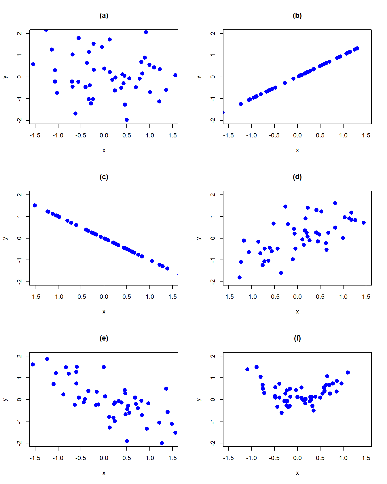
Figure 2.12: Probability scatterplots illustrating dependence between \(X\) and \(Y\).

Let \(X\) and \(Y\) be two random variables with \(E[X]=\mu_{X}\), \(\mathrm{var}(X)=\sigma_{X}^{2},E[Y]=\mu_{Y}\) and \(\mathrm{var}(Y)=\sigma_{Y}^{2}\).

Definition 2.21 The covariance between two random variables X and Y is given by: \[\begin{align*} \sigma_{XY} & =\mathrm{cov}(X,Y)=E[(X-\mu_{X})(Y-\mu_{Y})]\\ & =\sum_{x\in S_{X}}\sum_{y\in S_{Y}}(x-\mu_{X})(y-\mu_{Y})\Pr(X=x,Y=y)\textrm{ for discrete } X, Y ,\\ & =\int_{-\infty}^{\infty}\int_{-\infty}^{\infty}(x-\mu_{X})(y-\mu_{Y})p(x,y)~dx~dy\textrm{ for continuous } X, Y. \end{align*}\]

Definition 2.22 The correlation between two random variables X and Y is given by: \[ \rho_{XY}=\mathrm{cor}(X,Y)=\frac{\mathrm{cov}(X,Y)}{\sqrt{\mathrm{var}(X)\mathrm{var}(Y)}}=\frac{\sigma_{XY}}{\sigma_{X}\sigma_{Y}}. \] The correlation coefficient, \(\rho_{XY}\), is a scaled version of the covariance.

To see how covariance measures the direction of linear association, consider the probability scatterplot in Figure 2.13. In the figure, each pair of points occurs with equal probability. The plot is separated into quadrants (right to left, top to bottom). In the first quadrant (black circles), the realized values satisfy \(x<\mu_{X},y>\mu_{Y}\) so that the product \((x-\mu_{X})(y-\mu_{Y})<0\). In the second quadrant (blue squares), the values satisfy \(x>\mu_{X}\) and \(y>\mu_{Y}\) so that the product \((x-\mu_{X})(y-\mu_{Y})>0\). In the third quadrant (red triangles), the values satisfy \(x<\mu_{X}\) and \(y<\mu_{Y}\) so that the product \((x-\mu_{X})(y-\mu_{Y})>0\). Finally, in the fourth quadrant (green diamonds), \(x>\mu_{X}\) but \(y<\mu_{Y}\) so that the product \((x-\mu_{X})(y-\mu_{Y})<0\). Covariance is then a probability weighted average all of the product terms in the four quadrants. For the values in Figure 2.13, this weighted average is positive because most of the values are in the second and third quadrants.

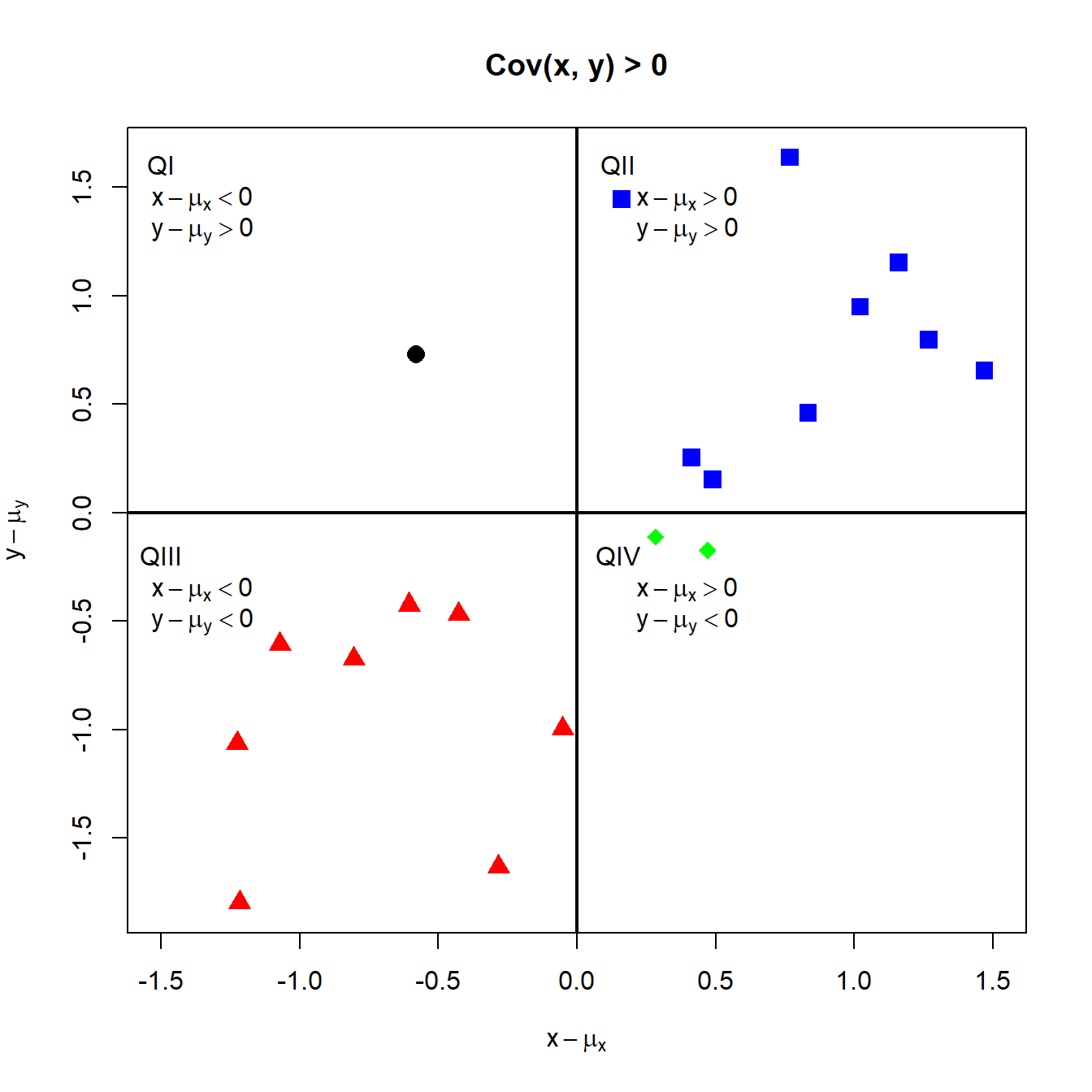
Figure 2.13: Probability scatterplot of discrete distribution with positive covariance. Each pair \((X,Y)\) occurs with equal probability.

Example 2.49 (Calculate covariance and correlation for discrete random variables)

For the data in Table 2.3, we have: \[\begin{gather*} \sigma_{XY}=\mathrm{cov}(X,Y)=(0-3/2)(0-1/2)\cdot1/8+(0-3/2)(1-1/2)\cdot0\\ +\cdots+(3-3/2)(1-1/2)\cdot1/8=1/4\\ \rho_{XY}=\mathrm{cor}(X,Y)=\frac{1/4}{\sqrt{(3/4)\cdot(1/2)}}=0.577 \end{gather*}\]

\(\blacksquare\)

2.2.4.1 Properties of covariance and correlation

Let \(X\) and \(Y\) be random variables and let \(a\) and \(b\) be constants. Some important properties of \(\mathrm{cov}(X,Y)\) are summarized in the following Proposition:

Proposition 2.6 1. \(\mathrm{cov}(X,X)=\mathrm{var}(X)\) 2. \(\mathrm{cov}(X,Y)=\mathrm{cov}(Y,X)\) 3. \(\mathrm{cov}(X,Y)=E[XY]-E[X]E[Y]=E[XY]-\mu_{X}\mu_{Y}\) 4. \(\mathrm{cov}(aX,bY)=a\cdot b\cdot\mathrm{cov}(X,Y)\) 5. If \(X\) and \(Y\) are independent then \(\mathrm{cov}(X,Y)=0\) (no association \(\Longrightarrow\) no linear association). However, if \(\mathrm{cov}(X,Y)=0\) then \(X\) and \(Y\) are not necessarily independent (no linear association \(\nRightarrow\) no association). 6. If \(X\) and \(Y\) are jointly normally distributed and \(\mathrm{cov}(X,Y)=0\), then \(X\) and \(Y\) are independent.

The first two properties are intuitive. The third property results from expanding the definition of covariance: \[\begin{align*} \mathrm{cov}(X,Y) & =E[(X-\mu_{X})(Y-\mu_{Y})]\\ & =E\left[XY-X\mu_{Y}-\mu_{X}Y+\mu_{X}\mu_{Y}\right]\\ & =E[XY]-E[X]\mu_{Y}-\mu_{X}E[Y]+\mu_{X}\mu_{Y}\\ & =E[XY]-2\mu_{X}\mu_{Y}+\mu_{X}\mu_{Y}\\ & =E[XY]-\mu_{X}\mu_{Y} \end{align*}\] The fourth property follows from the linearity of expectations: \[\begin{align*} \mathrm{cov}(aX,bY) & =E[(aX-a\mu_{X})(bY-b\mu_{Y})]\\ & =a\cdot b\cdot E[(X-\mu_{X})(Y-\mu_{Y})]\\ & =a\cdot b\cdot\mathrm{cov}(X,Y) \end{align*}\] The fourth property shows that the value of \(\mathrm{cov}(X,Y)\) depends on the scaling of the random variables \(X\) and \(Y\). By simply changing the scale of \(X\) or \(Y\) we can make \(\mathrm{cov}(X,Y)\) equal to any value that we want. Consequently, the numerical value of \(\mathrm{cov}(X,Y)\) is not informative about the strength of the linear association between \(X\) and \(Y\). However, the sign of \(\mathrm{cov}(X,Y)\) is informative about the direction of linear association between \(X\) and \(Y\).

The fifth property should be intuitive. Independence between the random variables \(X\) and \(Y\) means that there is no relationship, linear or nonlinear, between \(X\) and \(Y\). However, the lack of a linear relationship between \(X\) and \(Y\) does not preclude a nonlinear relationship.

The last result illustrates an important property of the normal distribution: lack of covariance implies independence.

Some important properties of \(\mathrm{cor}(X,Y)\) are:

Proposition 2.7 1. \(-1\leq\rho_{XY}\leq1\) 2. If \(\rho_{XY}=1\) then \(X\) and \(Y\) are perfectly positively linearly related. That is, \(Y=aX+b\) where \(a>0\). 3. If \(\rho_{XY}=-1\) then \(X\) and \(Y\) are perfectly negatively linearly related. That is, \(Y=aX+b\) where \(a<0\). 4. If \(\rho_{XY}=0\) then \(X\) and \(Y\) are not linearly related but may be nonlinearly related. 5. \(\mathrm{cor}(aX,bY)=\mathrm{cor}(X,Y)\) if \(a>0\) and \(b>0\); \(\mathrm{cor}(X,Y)=-\mathrm{cor}(X,Y)\) if \(a>0,b<0\) or \(a<0,b>0\).

TBD: discuss the results briefly

2.2.5 Bivariate normal distributions

Let \(X\) and \(Y\) be distributed bivariate normal. The joint pdf is given by: \[\begin{align} &f(x,y)=\frac{1}{2\pi\sigma_{X}\sigma_{Y}\sqrt{1-\rho_{XY}^{2}}}\times\tag{2.47}\\ &\exp\left\{ -\frac{1}{2(1-\rho_{XY}^{2})}\left[\left(\frac{x-\mu_{X}}{\sigma_{X}}\right)^{2}+\left(\frac{y-\mu_{Y}}{\sigma_{Y}}\right)^{2}-\frac{2\rho_{XY}(x-\mu_{X})(y-\mu_{Y})}{\sigma_{X}\sigma_{Y}}\right]\right\} \nonumber \end{align}\] where \(E[X]=\mu_{X}\), \(E[Y]=\mu_{Y}\), \(\mathrm{sd}(X)=\sigma_{X}\), \(\mathrm{sd}(Y)=\sigma_{Y}\), and \(\rho_{XY}=\mathrm{cor}(X,Y)\). The correlation coefficient \(\rho_{XY}\) describes the dependence between \(X\) and \(Y\). If \(\rho_{XY}=0\) then the pdf collapses to the pdf of the standard bivariate normal distribution. In this case, \(X\) and \(Y\) are independent random variables since \(f(x,y)=f(x)f(y).\)

It can be shown that the marginal distributions of \(X\) and \(Y\) are normal: \(X\sim N(\mu_{X},\sigma_{X}^{2})\), \(Y\sim N(\mu_{Y},\sigma_{Y}^{2})\). In addition, it can be shown that the conditional distributions \(f(x|y)\) and \(f(y|x)\) are also normal with means given by: \[\begin{align} \mu_{X|Y=y} & =\alpha_{X}+\beta_{X}\cdot y,\tag{2.48}\\ \mu_{Y|X=x} & =\alpha_{Y}+\beta_{Y}\cdot x,\tag{2.49} \end{align}\] where, \[\begin{align*} \alpha_{X} & =\mu_{X}-\beta_{X}\mu_{X},~\beta_{X}=\sigma_{XY}/\sigma_{Y}^{2},\\ \alpha_{Y} & =\mu_{Y}-\beta_{Y}\mu_{X},~\beta_{Y}=\sigma_{XY}/\sigma_{X}^{2}, \end{align*}\] and variances given by, \[\begin{align*} \sigma_{X|Y=y}^{2} & =\sigma_{X}^{2}-\sigma_{XY}^{2}/\sigma_{Y}^{2},\\ \sigma_{X|Y=y}^{2} & =\sigma_{Y}^{2}-\sigma_{XY}^{2}/\sigma_{X}^{2}. \end{align*}\] Notice that the conditional means (regression functions) (2.43) and (2.44) are linear functions of \(x\) and \(y\), respectively.

Example 2.50 (Expressing the bivariate normal distribution using matrix algebra)

The formula for the bivariate normal distribution (2.47) is a bit messy. We can greatly simplify the formula by using matrix algebra. Define the \(2\times1\) vectors \(\mathbf{x}=(x,y)^{\prime}\) and \(\mu=(\mu_{X},\mu_{y})^{\prime},\) and the \(2\times2\) matrix: \[ \Sigma=\left(\begin{array}{cc} \sigma_{X}^{2} & \sigma_{XY}\\ \sigma_{XY} & \sigma_{Y}^{2} \end{array}\right) \] Then the bivariate normal distribution (2.47) may be compactly expressed as: \[\begin{equation} f(\mathbf{x})=\frac{1}{2\pi\det(\Sigma)^{1/2}}e^{-\frac{1}{2}(\mathbf{x}-\mu)^{\prime}\Sigma^{-1}(\mathbf{x}-\mu)} \tag{2.50} \end{equation}\] where, \[\begin{align*} \det(\Sigma)&=\sigma_{X}^{2}\sigma_{Y}^{2}-\sigma_{XY}^{2}=\sigma_{X}^{2}\sigma_{Y}^{2}-\sigma_{X}^{2}\sigma_{Y}^{2}\rho_{XY}^{2}=\sigma_{X}^{2}\sigma_{Y}^{2}(1-\rho_{XY}^{2})\\ \Sigma^{-1} &= \frac{1}{\det(\Sigma)} \left(\begin{array}{cc} \sigma_{Y}^{2} & -\sigma_{XY}\\ -\sigma_{XY} & \sigma_{X}^{2} \end{array}\right) \end{align*}\]

\(\blacksquare\)

Example 2.51 (Plotting the bivariate normal distribution)

The R package mvtnorm contains the functions dmvnorm(), pmvnorm(), and qmvnorm() which can be used to compute the bivariate normal pdf, cdf and quantiles, respectively. Plotting the bivariate normal distribution over a specified grid of \(x\) and \(y\) values in R can be done with the persp() function. First, we specify the parameter values for the joint distribution. Here, we choose \(\mu_{X}=\mu_{Y}=0\), \(\sigma_{X}=\sigma_{Y}=1\) and \(\rho=0.5\). We will use the dmvnorm() function to evaluate the joint pdf at these values. To do so, we must specify a covariance matrix of the form: \[ \Sigma=\left(\begin{array}{cc} \sigma_{X}^{2} & \sigma_{XY}\\ \sigma_{XY} & \sigma_{Y}^{2} \end{array}\right)=\left(\begin{array}{cc} 1 & 0.5\\ 0.5 & 1 \end{array}\right). \] In R this matrix can be created using:

sigma = matrix(c(1, 0.5, 0.5, 1), 2, 2)

Next we specify a grid of \(x\) and \(y\) values between \(-3\) and \(3\):

x = seq(-3, 3, length=25)
y = seq(-3, 3, length=25)

To evaluate the joint pdf over the two-dimensional grid we can use the outer() function:

# function to evaluate bivariate normal pdf on grid
bv.norm <- function(x, y, sigma) {
  z = cbind(x,y)
  return(dmvnorm(z, sigma=sigma))
}
# use outer function to evaluate pdf on 2D grid of x-y values
fxy = outer(x, y, bv.norm, sigma)

To create the 3D plot of the joint pdf, use the persp() function:

persp(x, y, fxy, theta=60, phi=30, expand=0.5, ticktype="detailed", 
      zlab="f(x,y)",col="grey")

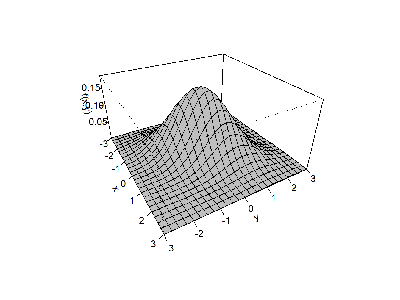
Figure 2.14: Bivariate normal pdf with \(\mu_{X}=\mu_{Y}=0\), \(\sigma_{X}\sigma_{Y}=1\) and \(\rho=0.5\).

The resulting plot is given in Figure 2.14.

\(\blacksquare\)

2.2.6 Expectation and variance of the sum of two random variables

Proposition 2.8 Let \(X\) and \(Y\) be two random variables with well defined means, variances and covariance and let \(a\) and \(b\) be constants. Then the following results hold: \[\begin{align} E[aX+bY] & =aE[X]+bE[Y]=a\mu_{X}+b\mu_{Y} \tag{2.51} \\ \mathrm{var}(aX+bY) & =a^{2}\mathrm{var}(X)+b^{2}\mathrm{var}(Y)+2\cdot a\cdot b\cdot\mathrm{cov}(X,Y)\\ & =a^{2}\sigma_{X}^{2}+b^{2}\sigma_{Y}^{2}+2\cdot a\cdot b\cdot\sigma_{XY} \tag{2.52} \end{align}\]

The first result (2.51) states that the expected value of a linear combination of two random variables is equal to a linear combination of the expected values of the random variables. This result indicates that the expectation operator is a linear operator. In other words, expectation is additive. The second result (2.52) states that variance of a linear combination of random variables is not a linear combination of the variances of the random variables. In particular, notice that covariance comes up as a term when computing the variance of the sum of two (not independent) random variables. Hence, the variance operator is not, in general, a linear operator. That is, variance, in general, is not additive.

It is instructive to go through the derivation of these results. Let \(X\) and \(Y\) be discrete random variables. Then, \[\begin{align*} E[aX+bY] & =\sum_{x\in S_{X}}\sum_{y\in S_{y}}(ax+by)\Pr (X=x,Y=y)\\ & =\sum_{x\in S_{X}}\sum_{y\in S_{y}}ax\Pr(X=x,Y=y)+\sum_{x\in S_{X}}\sum_{y\in S_{y}}bx\Pr(X=x,Y=y)\\ & =a\sum_{x\in S_{X}}x\sum_{y\in S_{y}}\Pr(X=x,Y=y)+b\sum_{y\in S_{y}}y\sum_{x\in S_{X}}\Pr(X=x,Y=y)\\ & =a\sum_{x\in S_{X}}x\Pr(X=x)+b\sum_{y\in S_{y}}y\Pr(Y=y)\\ & =aE[X]+bE[Y]=a\mu_{X}+b\mu_{Y}. \end{align*}\] The result for continuous random variables is similar. Effectively, the summations are replaced by integrals and the joint probabilities are replaced by the joint pdf.

Next, let \(X\) and \(Y\) be discrete or continuous random variables. Then, using the definition of variance we get: \[\begin{align*} \mathrm{var}(aX+bY) & =E[(aX+bY-E[aX+bY])^{2}]\\ & =E[(aX+bY-a\mu_{X}-b\mu_{Y})^{2}]\\ & =E[(a(X-\mu_{X})+b(Y-\mu_{Y}))^{2}]\\ & =a^{2}E[(X-\mu_{X})^{2}]+b^{2}E[(Y-\mu_{Y})^{2}]+2\cdot a\cdot b\cdot E[(X-\mu_{X})(Y-\mu_{Y})]\\ & =a^{2}\mathrm{var}(X)+b^{2}\mathrm{var}(Y)+2\cdot a\cdot b\cdot\mathrm{cov}(X,Y). \end{align*}\]

2.2.6.1 Linear combination of two normal random variables

The following proposition gives an important result concerning a linear combination of normal random variables.

Proposition 2.9 Let \(X\sim N(\mu_{X},\sigma_{X}^{2})\), \(Y\sim N(\mu_{Y},\sigma_{Y}^{2})\), \(\sigma_{XY}=\mathrm{cov}(X,Y)\) and \(a\) and \(b\) be constants. Define the new random variable \(Z\) as: \[ Z=aX+bY. \] Then, \[ Z\sim N(\mu_{Z},\sigma_{Z}^{2}), \] where \(\mu_{Z}=a\mu_{X}+b\mu_{Y}\) and \(\sigma_{Z}^{2}=a^{2}\sigma_{X}^{2}+b^{2}\sigma_{Y}^{2}+2ab\sigma_{XY}\).

This important result states that a linear combination of two normally distributed random variables is itself a normally distributed random variable. The proof of the result relies on the change of variables theorem from calculus and is omitted. Not all random variables have the nice property that their distributions are closed under addition.

Example 2.52 (Portfolio of two assets)

Consider a portfolio of two stocks \(A\) (Amazon) and \(B\) (Boeing) with investment shares \(x_{A}\) and \(x_{B}\) with \(x_{A}+x_{B}=1\). Let \(R_{A}\) and \(R_{B}\) denote the simple monthly returns on these assets, and assume that \(R_{A}\sim N(\mu_{A},\sigma_{A}^{2})\) and \(R_{B}\sim N(\mu_{B},\sigma_{B}^{2})\). Furthermore, let \(\sigma_{AB}=\rho_{AB}\sigma_{A}\sigma_{B}=\mathrm{cov}(R_{A},R_{B})\). The portfolio return is \(R_{p}=x_{A}R_{A}+x_{B}R_{B}\), which is a linear function of two random variables. Using the properties of linear functions of random variables, we have: \[\begin{align*} \mu_{p} & =E[R_{p}]=x_{A}E[R_{A}]+x_{B}E[R_{B}]=x_{A}\mu_{A}+x_{B}\mu_{B}\\ \sigma_{p}^{2} & =\mathrm{var}(R_{p})=x_{A}^{2}\mathrm{var}(R_{A})+x_{B}^{2}\mathrm{var}(R_{B})+2x_{A}x_{B}\mathrm{cov}(R_{A},R_{B})\\ & =x_{A}^{2}\sigma_{A}^{2}+x_{B}^{2}\sigma_{B}^{2}+2x_{A}x_{B}\sigma_{AB}. \end{align*}\]

\(\blacksquare\)