5.2 Time Series Descriptive Statistics
In this section, we consider graphical and numerical descriptive statistics for summarizing the linear time dependence in a time series.
5.2.1 Sample Autocovariances and Autocorrelations
For a covariance stationary time series process \(\{X_{t}\}\), the autocovariances \(\gamma_{j}=\mathrm{cov}(X_{t},X_{t-j})\) and autocorrelations \(\rho_{j}=\mathrm{cov}(X_{t},X_{t-j})/\sqrt{\mathrm{var}(X_{t})\mathrm{var}(X_{t-j})}=\gamma_{j}/\sigma^{2}\) describe the linear time dependencies in the process. For a sample of data \(\{x_{t}\}_{t=1}^{T}\), the linear time dependencies are captured by the sample autocovariances and sample autocorrelations: \[\begin{align*} \hat{\gamma}_{j} & =\frac{1}{T-1}\sum_{t=j+1}^{T}(x_{t}-\bar{x})(x_{t-j}-\bar{x}),~j=1,2,\ldots,T-J+1,\\ \hat{\rho}_{j} & =\frac{\hat{\gamma}_{j}}{\hat{\sigma}^{2}},~j=1,2,\ldots,T-J+1, \end{align*}\] where \(\hat{\sigma}^{2}\) is the sample variance (5.3). The sample autocorrelation function (SACF) is a plot of \(\hat{\rho}_{j}\) vs. \(j\), and gives a graphical view of the linear time dependencies in the observed data.
The R function acf() computes and plots the sample autocorrelations
\(\hat{\rho}_{j}\) of a time series for a specified number of lags.
For example, to compute \(\hat{\rho}_{j}\) for \(j=1,\ldots,5\) for
the monthly and daily returns on Microsoft use:
##
## Autocorrelations of series 'coredata(msftMonthlyRetS)', by lag
##
##      0      1      2      3      4      5
## 1.000 -0.193 -0.114 0.193 -0.139 -0.023##
## Autocorrelations of series 'coredata(msftDailyRetS)', by lag
##
## 0 1 2 3 4 5
## 1.000 -0.044 -0.018 -0.010 -0.042 0.018None of these sample autocorrelations are very big and indicate lack of linear time dependence in the monthly and daily returns.
Sample autocorrelations can also be visualized using the function
acf(). Figure 5.21 shows the SACF for the
monthly and daily returns on Microsoft and the S&P 500 created using:
par(mfrow=c(2,2))
acf(coredata(msftMonthlyRetS), main="msftMonthlyRetS", lwd=2)
acf(coredata(sp500MonthlyRetS), main="sp500MonthlyRetS", lwd=2)
acf(coredata(msftDailyRetS), main="msftDailyRetS", lwd=2)
acf(coredata(sp500DailyRetS), main="sp500DailyRetS", lwd=2)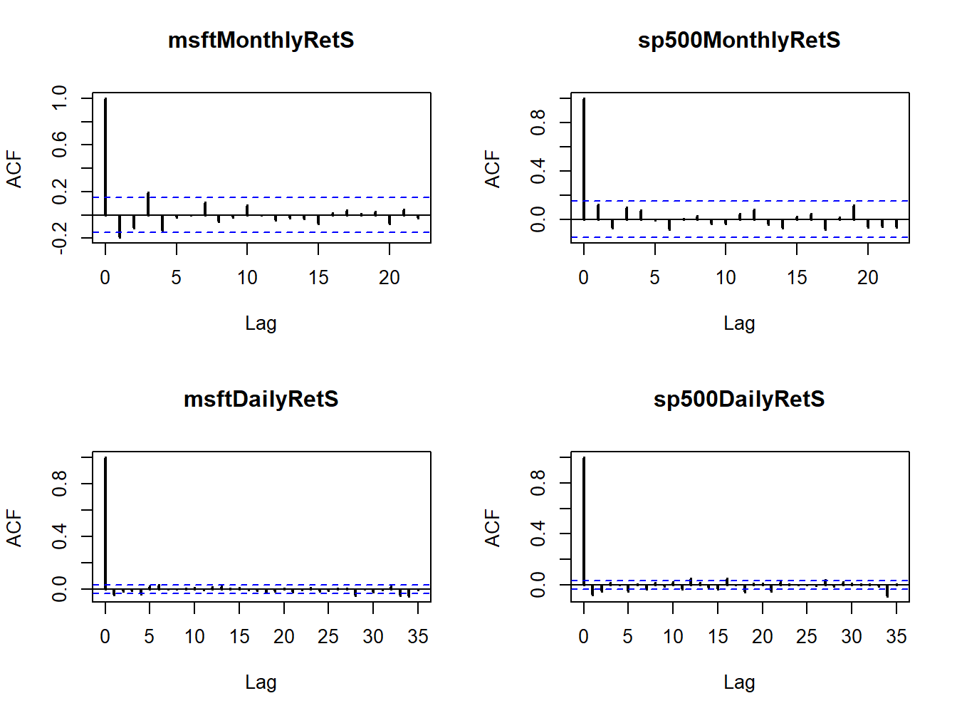
Figure 5.21: SACFs for the monthly and daily returns on Microsoft and the S&P 500 index.
None of the series show strong evidence for linear time dependence. The monthly returns have slightly larger sample autocorrelations at low lags than the daily returns. The dotted lines on the SACF plots are 5% critical values for testing the null hypothesis that the true autocorrelations \(\rho_{j}\) are equal to zero (see chapter 9). If \(\hat{\rho}_{j}\) crosses the dotted line then the null hypothesis that \(\rho_{j}=0\) can be rejected at the 5% significance level.
\(\blacksquare\)
5.2.2 Time dependence in volatility
The daily and monthly returns of Microsoft and the S&P 500 index do not exhibit much evidence for linear time dependence. Their returns are essentially uncorrelated over time. However, the lack of autocorrelation does not mean that returns are independent over time. There can be nonlinear time dependence. Indeed, there is strong evidence for a particular type of nonlinear time dependence in the daily returns of Microsoft and the S&P 500 index that is related to time varying volatility. This nonlinear time dependence, however, is less pronounced in the monthly returns.
Let \(y_{t}\sim\mathrm{GWN}(0,\sigma^{2})\). Then \(y_{t}\) is, by construction, independent over time. This implies that any function of \(y_{t}\) is also independent over time. To illustrate, Figure 5.22 shows \(y_{t}\), \(y_{t}^{2}\) and \(|y_{t}|\) together with their SACFs where \(y_{t}\sim \mathrm{GWN}(0,1)\) for \(t=1,\ldots,500\). Notice that all of the sample autocorrelations are essentially zero which confirms the lack of linear time dependence in \(y_{t}\), \(y_{t}^{2}\) and \(|y_{t}|\).
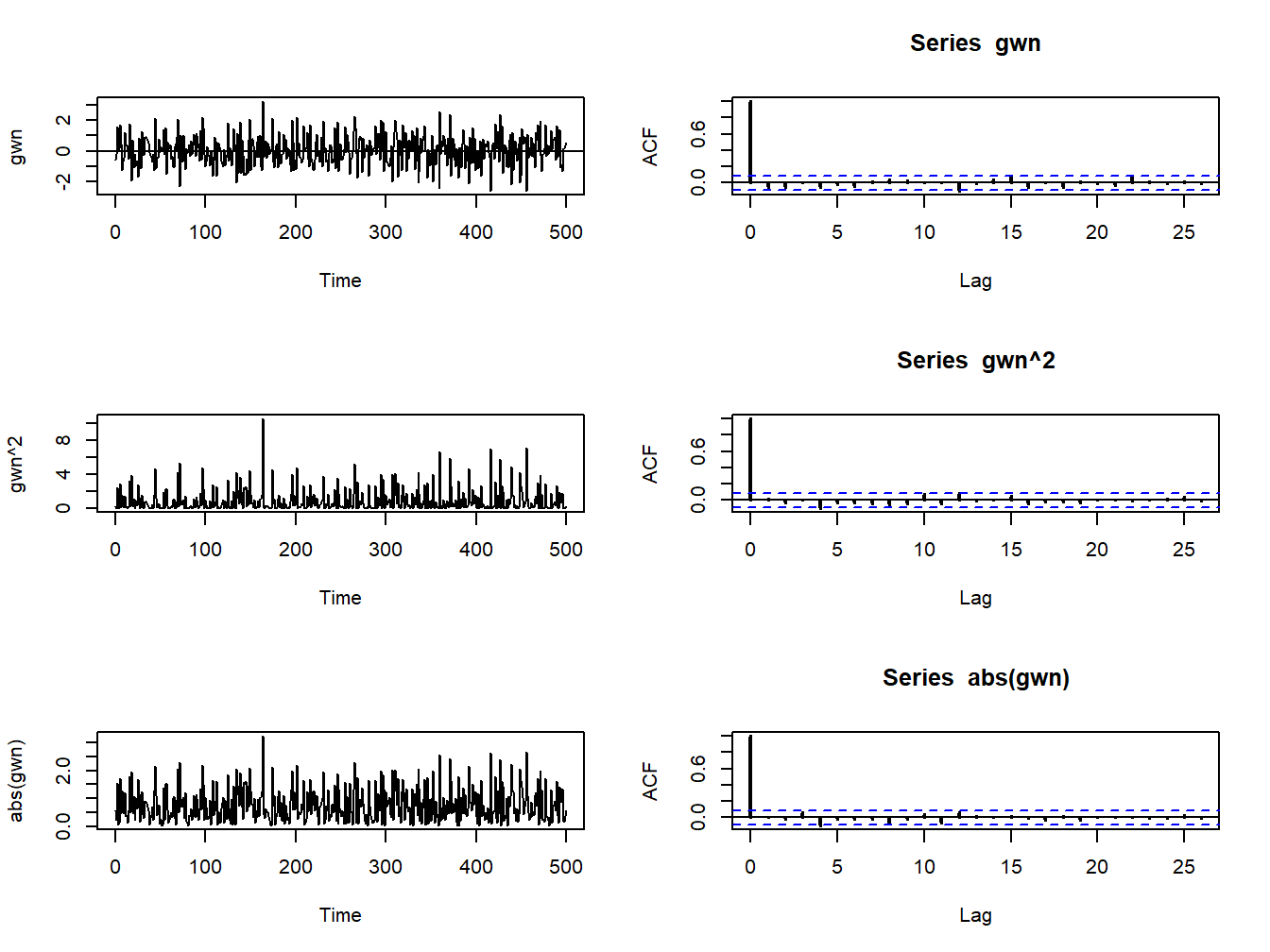
Figure 5.22: The left panel (top to bottom) shows \(y_{t}\), \(y_{t}^{2}\) and \(|y_{t}|\) where \(y_{t}\) is similar to GWN(0,1) for \(t=1,...,500.\) The right panel shows the corresponding SACFs.
\(\blacksquare\)
5.2.2.1 Nonlinear time dependence in asset returns
Figures 5.5 and 5.2 show that the daily and monthly returns on Microsoft and the S&P 500 index appear to exhibit periods of volatility clustering. That is, high periods of volatility tend to be followed by periods of high volatility and periods of low volatility appear to be followed by periods of low volatility. In other words, the volatility of the returns appears to exhibit some time dependence. This time dependence in volatility causes linear time dependence in the absolute value and squared value of returns.
To illustrate nonlinear time dependence in asset returns, Figure 5.23 shows the daily returns, absolute returns and squared returns for the S&P 500 index. Notice how the absolute and squared returns are large (small) when the daily returns are more (less) volatile. Figure 5.24 shows the SACFs for the absolute and squared daily and monthly returns. There is clear evidence of time dependence in the daily absolute and squared returns while there is some evidence of time dependence in the monthly absolute and squared returns. Since the absolute and squared daily returns reflect the volatility of the daily returns, the SACFs show a strong positive linear time dependence in daily return volatility.
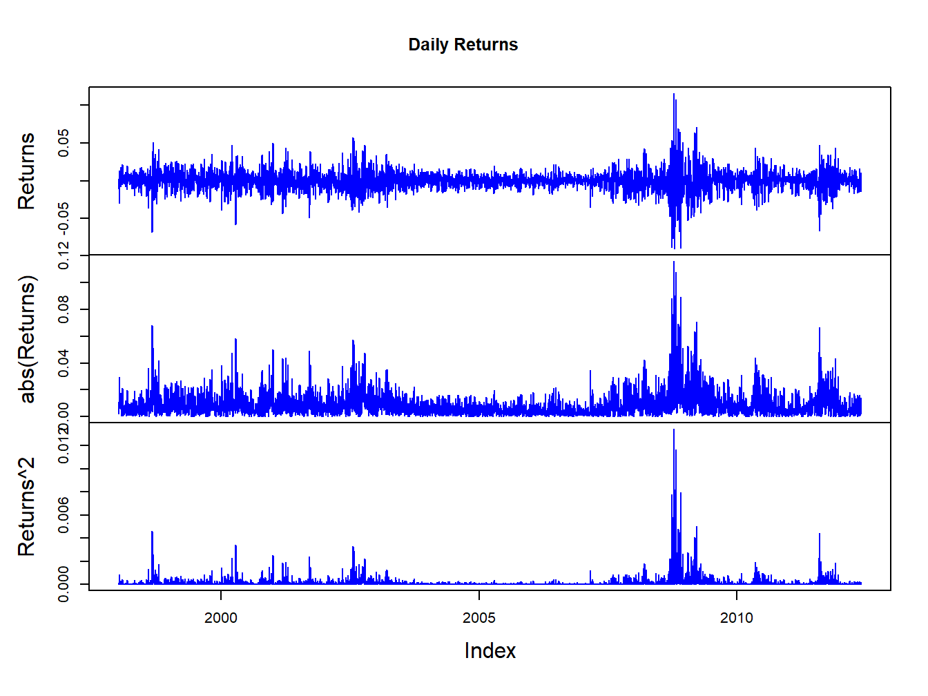
Figure 5.23: Daily returns, absolute returns, and squared returns on the S&P 500 index.
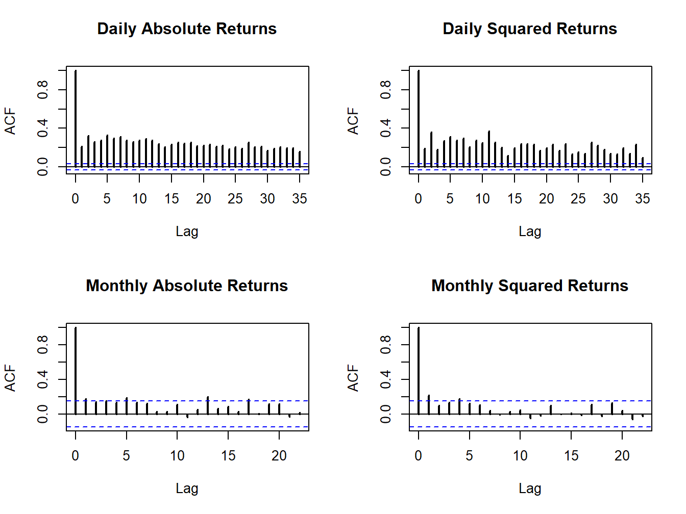
Figure 5.24: SACFs of daily and monthly absolute and squared returns on the S&P 500 index.
\(\blacksquare\)