1.4 Return Calculations with Data in R
This section discusses representing time series data in R using xts objects,
the calculation of returns from historical prices in R, as well as the graphical display of prices and returns.
1.4.1 Representing time series data using xts objects
The examples in this section are based on the daily adjusted closing price
data for Microsoft and Starbucks stock over the period January 4, 1993
through December 31, 20145. These data are available as the xts
objects msftDailyPrices and sbuxDailyPrices in the R package
IntroCompFinR6
suppressPackageStartupMessages(library(IntroCompFinR))
suppressPackageStartupMessages(library(xts))
suppressPackageStartupMessages(library(methods))
data(msftDailyPrices, sbuxDailyPrices)
head(cbind(msftDailyPrices,sbuxDailyPrices), 3)
## MSFT SBUX
## 1993-01-04 1.89 1.08
## 1993-01-05 1.92 1.10
## 1993-01-06 1.98 1.12## [1] "xts" "zoo"There are many different ways of representing a time series of data in R. For financial
time series xts (extensible time series) objects from the xts package are especially
convenient and useful. An xts object consists of two pieces of information: (1) a matrix of numeric data with different time series in the columns, (2) an R object representing the common time indexes associated with the rows of the data. xts objects extend and enhance the zoo
class of time series objects from the zoo package written by Achim Zeileis (zoo stands
for Z’s ordered observations).
The matrix of time series data can be extracted from the xts object using the xts function coredata():
## MSFT
## [1,] 1.89
## [2,] 1.92
## [3,] 1.98The resulting matrix of data does not have any date information. The date index can be
extracted using the xts function index():
## [1] "1993-01-04" "1993-01-05" "1993-01-06"The object date.index is of class Date:
## [1] "Date"When a Date object is printed, the date is displayed in the format yyyy-mm-dd.
However, internally each date represents the number of days since January 1, 1970:
## [1] 8404Here, 1993-01-04 (January 4, 1993) is \(8,404\) days after January 1, 1970. This allows
for simple date arithmetic (e.g. adding and subtracting dates, etc). More sophisticated
date arithmetic is available using the functions in the lubridate package.
There are several advantages of using xts objects to represent financial time series data. Most
financial time series do not follow an equally spaced regular calendar. The time index of a xts
object can be any strictly increasing date sequence which can match the times and dates for which assets trade on an exchange. For example, assets traded on the main US stock exchanges (e.g. NYSE and NASDAQ) trade only on weekdays between 9:30AM and 4:00PM Eastern Standard Time and do not trade on a number of holidays.
Another advantage of xts objects is that you can easily extract observations at or between specific dates. For example, to extract the daily price on January 3, 2014 use
## MSFT
## 2014-01-03 35.67To extract prices between January 3, 2014 and January 7, 2014, use
## MSFT
## 2014-01-03 35.67
## 2014-01-06 34.92
## 2014-01-07 35.19Or to extract all of the prices for January, 2014 use:
## MSFT
## 2014-01-02 35.91
## 2014-01-03 35.67
## 2014-01-06 34.92
## 2014-01-07 35.19
## 2014-01-08 34.56
## 2014-01-09 34.34
## 2014-01-10 34.83
## 2014-01-13 33.81
## 2014-01-14 34.58
## 2014-01-15 35.53
## 2014-01-16 35.65
## 2014-01-17 35.16
## 2014-01-21 34.96
## 2014-01-22 34.73
## 2014-01-23 34.85
## 2014-01-24 35.58
## 2014-01-27 34.82
## 2014-01-28 35.05
## 2014-01-29 35.43
## 2014-01-30 35.62
## 2014-01-31 36.57Two or more xts objects can be merged together and aligned to a common date index
using the xts function merge():
##            MSFT SBUX
## 1993-01-04 1.89 1.08
## 1993-01-05 1.92 1.10
## 1993-01-06 1.98 1.12If two or more xts objects have a common date index then they can be combined using cbind().
1.4.1.1 Basic calculations on xts objects.
Because xts objects typically contain a matrix of numeric data, many R functions that operate on matrices also operate on xts objects. For example, to transform msftDailyPrices to log prices use
##                 MSFT
## 1993-01-04 0.6365768
## 1993-01-05 0.6523252
## 1993-01-06 0.6830968
If two or more xts objects have the same time index then they can be added, subtracted, multiplied, and divided. For example,
msftPlusSbuxDailyPrices = msftDailyPrices + sbuxDailyPrices
colnames(msftPlusSbuxDailyPrices) = "MSFT+SBUX"
head(msftPlusSbuxDailyPrices,3)
## MSFT+SBUX
## 1993-01-04 2.97
## 1993-01-05 3.02
## 1993-01-06 3.10To compute the average of the Microsoft daily prices use
## [1] 19.85533If an R function, for some unknown reason, is not operating correctly on an xts object
first extract the data using coredata() and then call the R function. For example,
## [1] 19.855331.4.1.2 Changing the frequency of an xts object
Data at the daily frequency is the highest frequency of data considered in this book.
However, in many of the examples we want to use data at the weekly or monthly frequency. The
conversion of data at a daily frequency to data at a monthly frequency is easy to
do with xts objects. For example, end-of-month prices can be extracted from the daily prices using the xts function to.monthly():
msftMonthlyPrices = to.monthly(msftDailyPrices, OHLC=FALSE)
sbuxMonthlyPrices = to.monthly(sbuxDailyPrices, OHLC=FALSE)
msftSbuxMonthlyPrices = to.monthly(msftSbuxDailyPrices, OHLC=FALSE)
head(msftMonthlyPrices, 3)
## MSFT
## Jan 1993 1.92
## Feb 1993 1.85
## Mar 1993 2.06By default, to.monthly() extracts the data for the last day of the month and creates
a zoo yearmon date index. For monthly data, the yearmon date index is
convenient for printing and plotting as the month and year are nicely printed. To
preserve the Date class of the time index and show the end-of-month date, use the
optional argument indexAt = "lastof" in the call to to.monthly():
##            MSFT
## 1993-01-31 1.92
## 1993-02-28 1.85
## 1993-03-31 2.06
In the above calls to to.monthly(), the optional argument OHLC=FALSE prevents the creation of open, high, low, and closing prices for the month.
In a similar fashion, you can extract end-of-week prices using the xts function to.weekly():
msftWeeklyPrices = to.weekly(msftDailyPrices, OHLC=FALSE, indexA="lastof")
head(msftWeeklyPrices, 3)
## MSFT
## 1993-01-08 1.94
## 1993-01-15 2.00
## 1993-01-22 1.99Here, the weekly data are the closing prices on each Friday of the week:
## [1] "Friday" "Friday" "Friday"1.4.1.3 Plotting xts objects with plot.xts() and plot.zoo
Time plots of xts objects can be created with the generic plot()
function as there is a method function in the xts package for
objects of class xts. For example, Figure
1.1 shows a basic time plot of the
monthly closing prices of Microsoft and Starbucks created with:
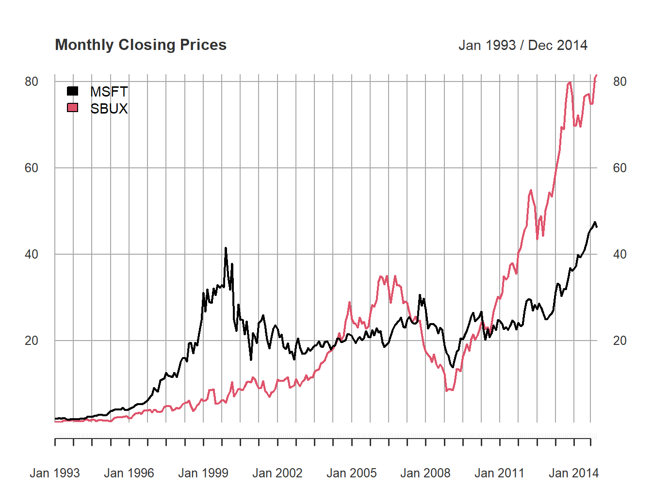
Figure 1.1: Single panel plot (default) with plot.xts()
The default plot style in plot.xts() is a single-panel plot with
multiple series. You can also create multi-panel plots, as in Figure
1.2, by setting the optional argument
multi.panel = TRUE in the call to plot.xts()
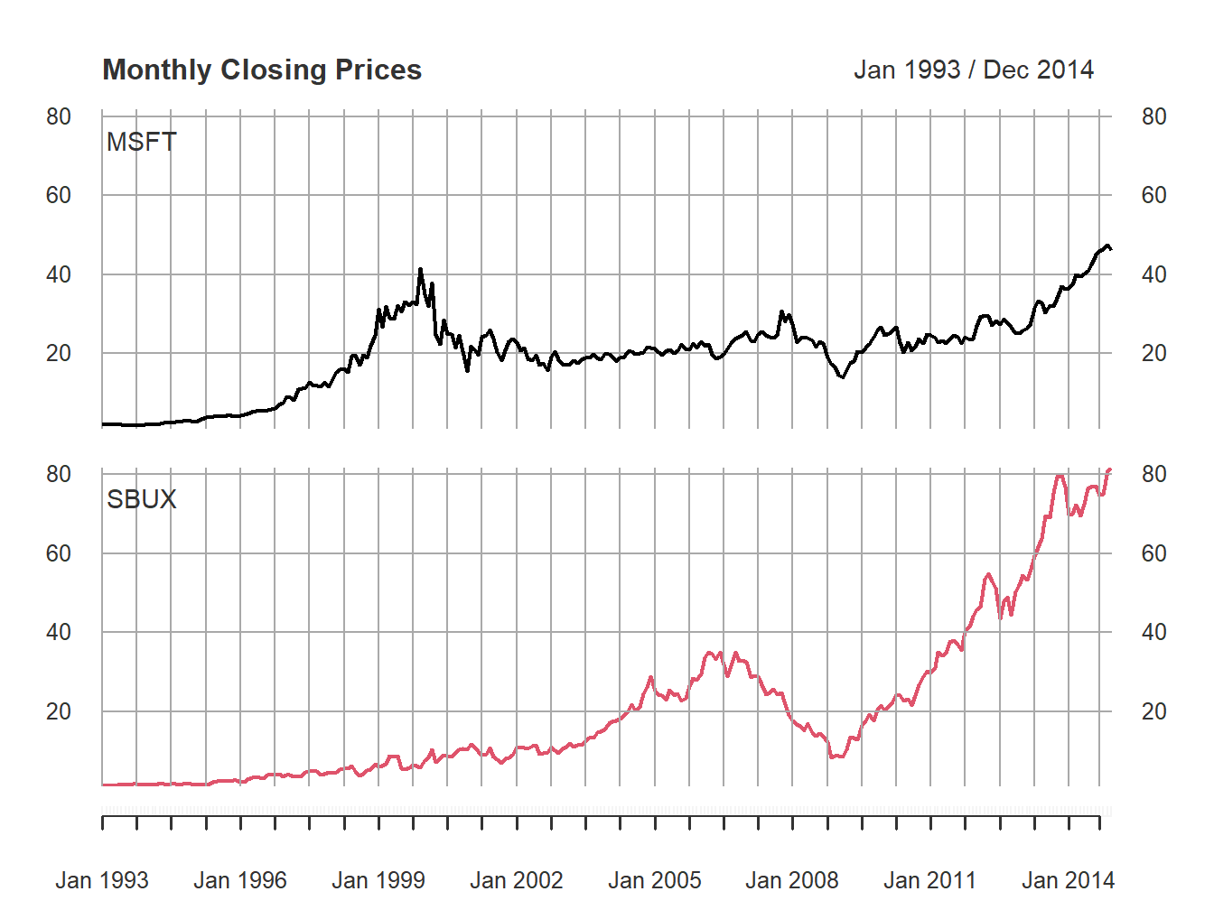
Figure 1.2: Multi-panel time series plot with plot.xts()
See the help file for plot.xts() for more examples of plotting xts objects.
Because the xts class inherits from the zoo class, the zoo
method function plot.zoo() can also be used to plot xts objects.
Figure 1.3 is created with
plot.zoo(msftSbuxMonthlyPrices, plot.type="single",
         main="Monthly Closing Prices",
         lwd = 2, col=c("black", "red"), ylab="Price")
grid()
legend(x="topleft", legend=colnames(msftSbuxMonthlyPrices),
      lwd = 2, col=c("black", "red"))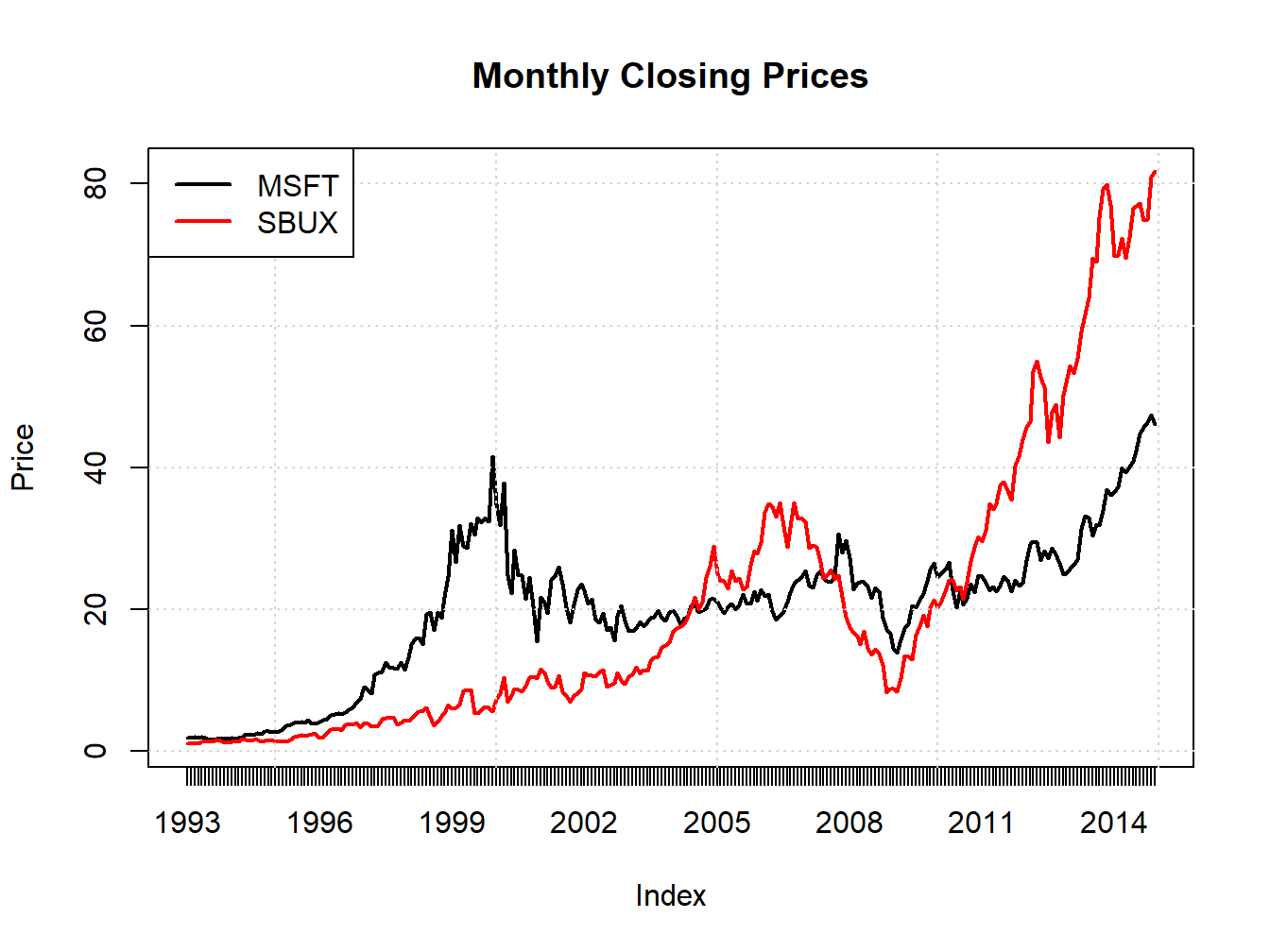
Figure 1.3: Single panel time series plot (default) with plot.zoo()
A muti-panel plot, shown in Figure 1.4, can be created using
plot.zoo(msftSbuxMonthlyPrices, plot.type="multiple", main="",
         lwd = 2, col=c("black", "red"), cex.axis=0.8)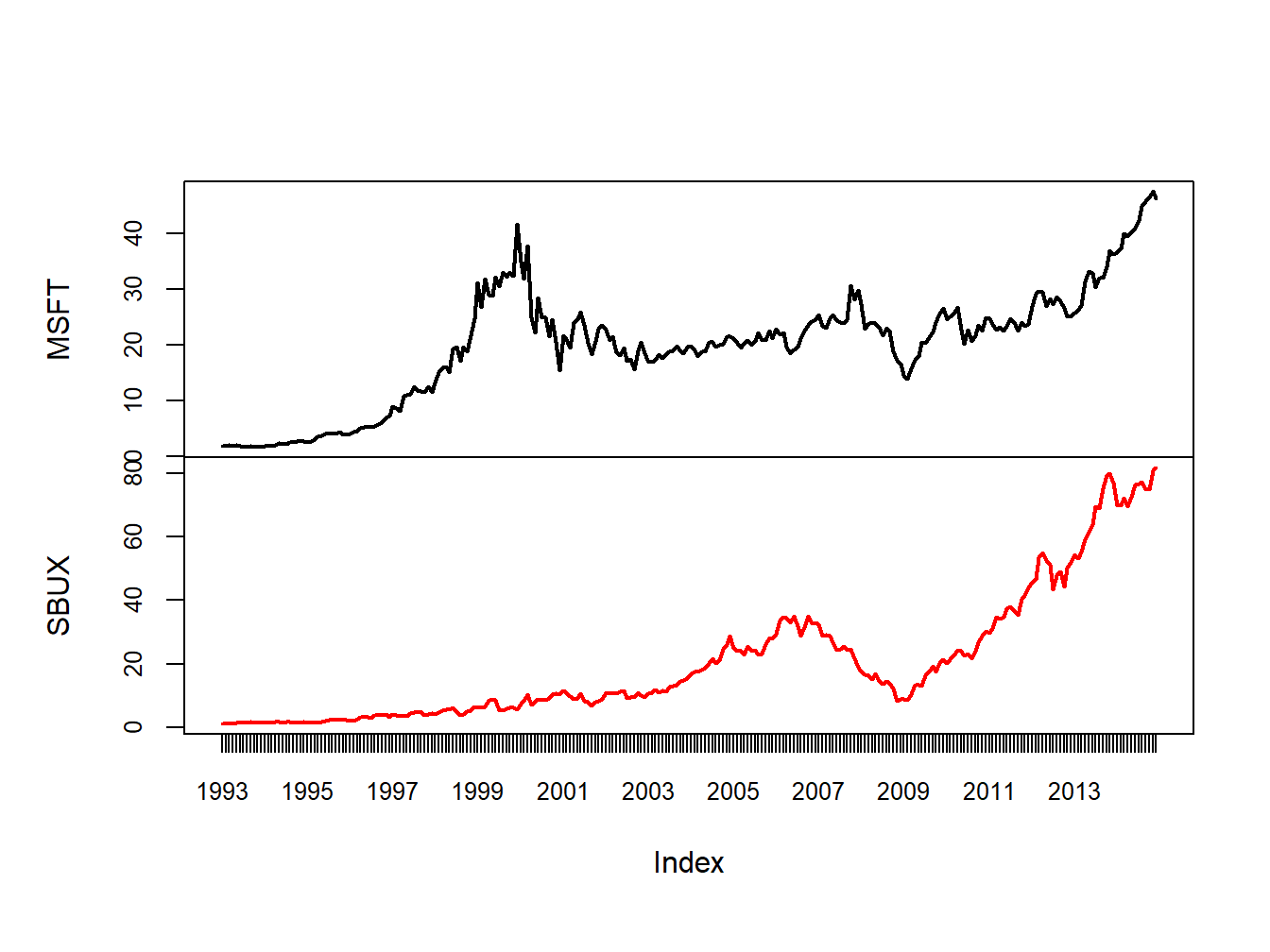
Figure 1.4: Multi-panel time series plot with plot.zoo()
Creating plots with plot.zoo() is a bit more involved than with plot.xts(), as
plot.xts() is newer. See the help file for plot.zoo() for more examples.
1.4.1.4 Ploting xts objects using autoplot() from ggplot2
The plots created using plot.xts() and plot.zoo() are created using the base
graphics system in R. This allows for a lot of flexibility but often the resulting
plots do not look very exciting or modern. In addition, these functions are not
well suited for plotting many time series together in a single plot.
Another very popular graphics system in R is provided by the ggplot2 package by
Hadley Wickham of RStudio. For plotting xts objects, especially with multiple
columns (data series), the ggplot2 function autoplot() is especially
convenient and easy:
library(ggplot2)
autoplot(msftSbuxDailyPrices, facets = NULL) +
  ggtitle("Daily Closing Prices") +
  ylab("Closing Price Per Share") +
  xlab("Year")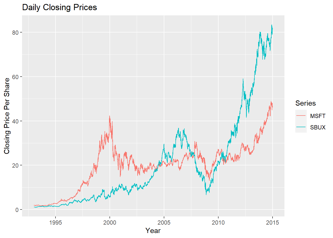
The syntax for creating graphs with autoplot() uses the grammar of graphics
syntax from the ggplot2 package. See the R Graphics Cookbook
for more details and examples on using the ggplot2 package. The call to autoplot()
first invokes the method function autoplot.zoo() from the zoo package and
creates a basic time series plot. Additional layers showing a main title and axes
labels are added using +. The optional argument facets = NULL specifies that
all series are plotted together on a single plot with different colors.
To produce a multi-panel plot call autoplot() with facets = Series ~ .:
autoplot(msftSbuxDailyPrices, facets = Series ~ .) +
  ggtitle("Daily Closing Prices") +
  ylab("Closing Price Per Share") +
  xlab("Year")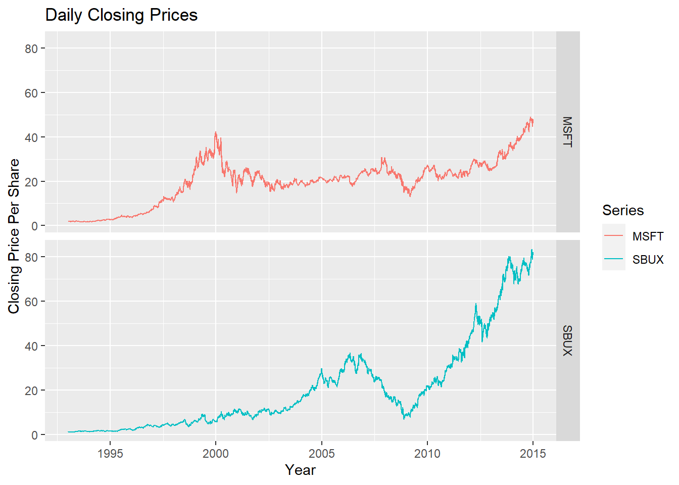
See the help file for autoplot.zoo() for more examples.
1.4.2 Calculating returns
In this sub-section, we illustrate how to calculate a time series of returns from a time series of prices.
1.4.2.1 Brute force return calculations
Consider computing simple monthly returns, \(R_{t}=\frac{P_{t}-P_{t-1}}{P_{t-1}}\),
from historical prices using the xts object sbuxMonthlyPrices. The R code for
a brute force calculation is:
##                 SBUX
## Jan 1993          NA
## Feb 1993 -0.06250000
## Mar 1993  0.04761905
Here, the diff() function computes the first difference in the prices,
\(P_{t}-P_{t-1}\), and the lag() function computes the lagged price,
\(P_{t-1}.\)7 An equivalent calculation is
\(R_{t}=\frac{P_{t}}{P_{t-1}}-1\):
##                 SBUX
## Jan 1993          NA
## Feb 1993 -0.06250000
## Mar 1993  0.04761905
Notice that the return for January, 1993 is NA (missing value). To
automatically remove this missing value, use the R function na.omit()
or explicitly exclude the first observation:
##                 SBUX
## Feb 1993 -0.06250000
## Mar 1993  0.04761905
## Apr 1993 0.01818182## SBUX
## Feb 1993 -0.06250000
## Mar 1993 0.04761905
## Apr 1993 0.01818182To compute continuously compounded returns from simple returns, use:
##                 SBUX
## Feb 1993 -0.06453852
## Mar 1993  0.04652002
## Apr 1993  0.01801851
Or, equivalently, to compute continuously compounded returns directly from prices, use:
##                 SBUX
## Feb 1993 -0.06453852
## Mar 1993  0.04652002
## Apr 1993  0.01801851
The above calculations used an xts object with a single column. If an xts
object has multiple columns the same calculations work for each column. For example,
msftSbuxMonthlyReturns = diff(msftSbuxMonthlyPrices)/lag(msftSbuxMonthlyPrices)
head(msftSbuxMonthlyReturns, n=3)
## MSFT SBUX
## Jan 1993 NA NA
## Feb 1993 -0.03645833 -0.06250000
## Mar 1993 0.11351351 0.04761905Also,
## MSFT SBUX
## Jan 1993 NA NA
## Feb 1993 -0.03713955 -0.06453852
## Mar 1993 0.10752034 0.04652002These are examples of vectorized calculations. That is, the calculations are performed on all columns simultaneously. This is computationally more efficient than looping the same calculation for each column. In R, you should try to vectorize calculations whenever possible.
1.4.2.2 Calculating returns using Return.calculate()
Simple and continuously compounded returns can be computed using the
PerformanceAnalytics function Return.calculate():
suppressPackageStartupMessages(library(PerformanceAnalytics))
# Simple returns
sbuxMonthlyReturns = Return.calculate(sbuxMonthlyPrices)
head(sbuxMonthlyReturns, n=3)## SBUX
## Jan 1993 NA
## Feb 1993 -0.06250000
## Mar 1993 0.04761905# CC returns
sbuxMonthlyReturnsC = Return.calculate(sbuxMonthlyPrices, method="log")
head(sbuxMonthlyReturnsC, n=3)## SBUX
## Jan 1993 NA
## Feb 1993 -0.06453852
## Mar 1993 0.04652002Return.calculate() also works with xts objects with multiple columns:
##                 MSFT        SBUX
## Jan 1993          NA          NA
## Feb 1993 -0.03645833 -0.06250000
## Mar 1993 0.11351351 0.04761905The advantages of using Return.calculate() instead of brute force calculations are: (1) clarity of code (you know what is being computed), (2) the same function is used for both simple and continuously compounded returns, (3) built-in error checking.
1.4.2.3 Equity curves
To directly compare the investment performance of two or more assets, plot the simple multi-period cumulative returns of each asset on the same graph. This type of graph, sometimes called an equity curve, shows how a one dollar investment amount in each asset grows over time. Better performing assets have higher equity curves. For simple returns, the k-period returns are \(R_{t}(k)=\prod\limits _{j=0}^{k-1}(1+R_{t-j})\) and represent the growth of one dollar invested for \(k\) periods. For continuously compounded returns, the k-period returns are \(r_{t}(k)=\sum\limits _{j=0}^{k-1}r_{t-j}\). However, this continuously compounded \(k\)-period return must be converted to a simple \(k\)-period return, using \(R_{t}(k)=\exp\left(r_{t}(k)\right)-1\), to properly represent the growth of one dollar invested for \(k\) periods.
To create the equity curves for Microsoft and Starbucks based on simple returns use:8
msftMonthlyReturns = na.omit(Return.calculate(msftMonthlyPrices))
sbuxMonthlyReturns = na.omit(Return.calculate(sbuxMonthlyPrices))
equityCurveMsft = cumprod(1 + msftMonthlyReturns)
equityCurveSbux = cumprod(1 + sbuxMonthlyReturns)
dataToPlot = merge(equityCurveMsft, equityCurveSbux)
plot(dataToPlot, main="Monthly Equity Curves", legend.loc="topleft")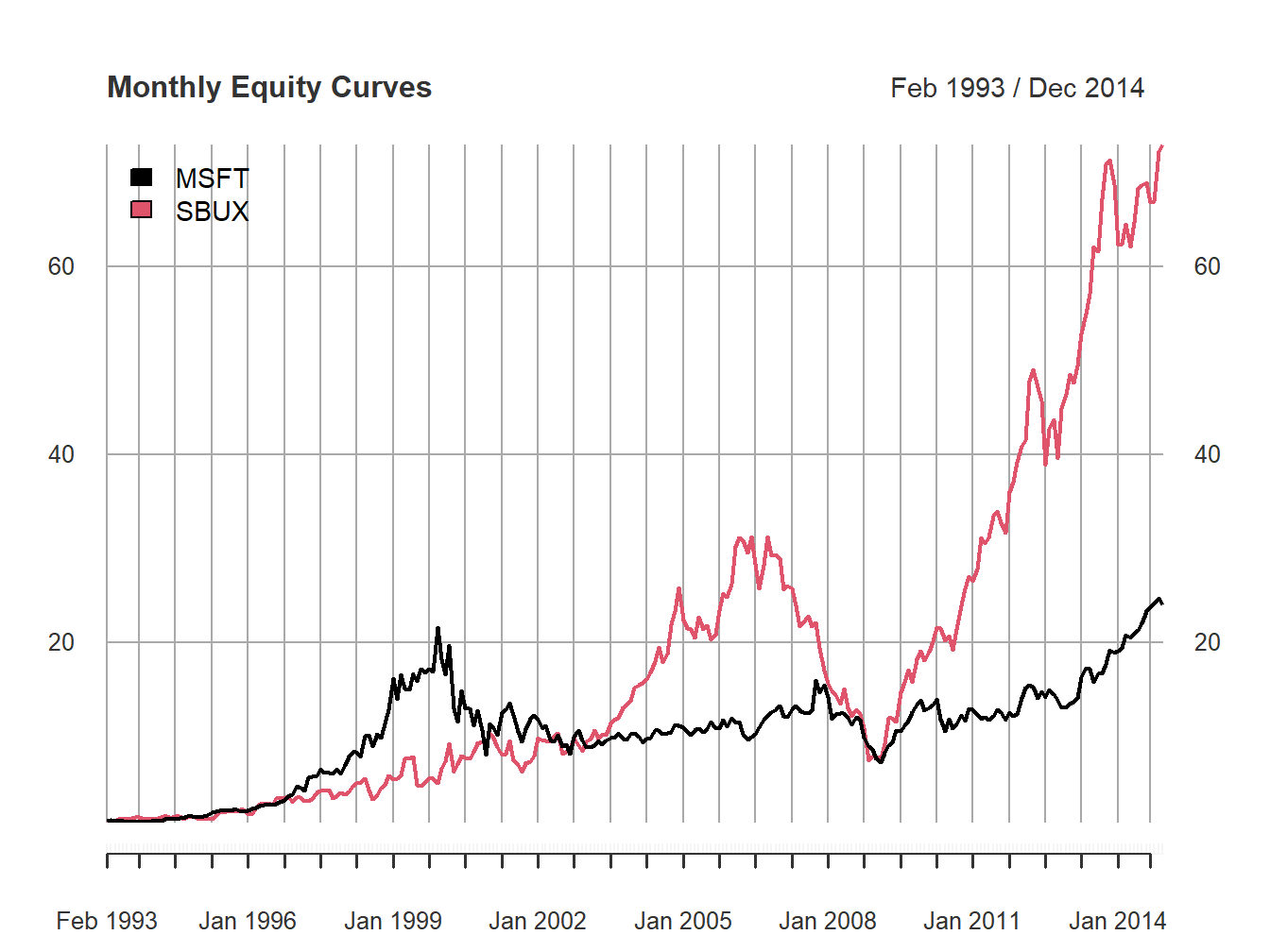
Figure 1.5: Monthly equity curve for Microsoft and Starbucks.
The R function cumprod() creates the cumulative products
needed for the equity curves. Figure 1.5
shows that a one dollar investment in Starbucks dominated a one dollar
investment in Microsoft over the given period. In particular,
$1 invested in Microsoft grew to about only $22 (over about 20 years)
whereas $1 invested in Starbucks grew over $70.
Notice the huge increases and decreases in value of Microsoft during
the dot-com bubble and bust over the period 1998 - 2001, and the enormous increase in value of Starbucks from 2009 - 2014.
\(\blacksquare\)
1.4.3 Calculating portfolio returns from time series data
As discussed in sub-section 1.3, the calculation of portfolio returns depends on the assumptions made about the portfolio weights over time.
1.4.3.1 Constant portfolio weights
The easiest case assumes that portfolio weights are constant over time. To illustrate, consider an equally weighted portfolio of Microsoft and Starbucks stock. A time series a portfolio monthly returns can be created directly from the monthly returns on Microsoft and Starbucks stock:
x.msft = x.sbux = 0.5
msftMonthlyReturns = na.omit(Return.calculate(msftMonthlyPrices))
sbuxMonthlyReturns = na.omit(Return.calculate(sbuxMonthlyPrices))
equalWeightPortMonthlyReturns = x.msft*msftMonthlyReturns +
  x.sbux*sbuxMonthlyReturns
head(equalWeightPortMonthlyReturns, 3)
## MSFT
## Feb 1993 -0.04947917
## Mar 1993 0.08056628
## Apr 1993 -0.02974404The same calculation can be performed using the PerformanceAnalytics function
Return.portfolio():
equalWeightPortMonthlyReturns =
  Return.portfolio(na.omit(msftSbuxMonthlyReturns),
                   weights = c(x.msft, x.sbux),
                   rebalance_on = "months")
head(equalWeightPortMonthlyReturns, 3)
## portfolio.returns
## Feb 1993 -0.04947917
## Mar 1993 0.08056628
## Apr 1993 -0.02974404Here, the optional argument rebalance_on = "months" specifies that the portfolio
is to be rebalanced to the specified weights at the beginning of every month.
If you also want the asset contributions to the portfolio return set the
optional argument contribution = TRUE (recall, asset contributions sum to the
portfolio return):
equalWeightPortMonthlyReturns =
  Return.portfolio(na.omit(msftSbuxMonthlyReturns),
                   weights = c(x.msft, x.sbux),
                   rebalance_on = "months",
                   contribution = TRUE)
head(equalWeightPortMonthlyReturns, 3)
## portfolio.returns MSFT SBUX
## Feb 1993 -0.04947917 -0.01822917 -0.031250000
## Mar 1993 0.08056628 0.05675676 0.023809524
## Apr 1993 -0.02974404 -0.03883495 0.009090909You can see the rebalancing calculations by setting the optional argument verbose = TRUE:
equalWeightPortMonthlyReturns =
  Return.portfolio(na.omit(msftSbuxMonthlyReturns),
                   weights = c(x.msft, x.sbux),
                   rebalance_on = "months",
                   verbose = TRUE)
names(equalWeightPortMonthlyReturns)
## [1] "returns" "contribution" "BOP.Weight" "EOP.Weight" "BOP.Value"
## [6] "EOP.Value"In this case Return.portfolio() returns a list with the above components. The
component BOP.Weight shows the beginning-of-period portfolio weights, and the
component EOP.Weight shows the end-of-period portfolio weights (before any rebalancing).
##          MSFT SBUX
## Feb 1993  0.5  0.5
## Mar 1993  0.5  0.5
## Apr 1993  0.5  0.5
With monthly returns and with rebalance_on = "months", the beginning-of-period
weights are always rebalanced to the initially supplied weights.
##               MSFT      SBUX
## Feb 1993 0.5068493 0.4931507
## Mar 1993 0.5152454 0.4847546
## Apr 1993 0.4753025 0.5246975
Because the returns for Microsoft and Starbux are different every month the end-of-period weights drift away from the beginning-of-period weights.
1.4.3.2 Buy-and-hold portfolio
In the buy-and-hold portfolio, no rebalancing of the initial portfolio is done
and the portfolio weights are allowed to evolve over time based on the returns
of the assets. Hence, the computation of the portfolio return each month requires
knowing the weights on each asset each month. You can use Return.portfolio() to
compute the buy-and-hold portfolio returns as follows:
buyHoldPortMonthlyReturns =
  Return.portfolio(na.omit(msftSbuxMonthlyReturns),
                   weights = c(x.msft, x.sbux))
head(buyHoldPortMonthlyReturns, 3)
## portfolio.returns
## Feb 1993 -0.04947917
## Mar 1993 0.08101761
## Apr 1993 -0.03186097Omitting the optional argument rebalance_on tells Return.portfolio() to not
rebalance the portfolio at all (default behavior of the function).
1.4.3.3 Periodic rebalancing
In practice, a portfolio may be rebalanced at a specific frequency that is different than the frequency of the returns. For example, with monthly returns the portfolio might be rebalanced quarterly or annually. For example, to rebalance the equally weighted portfolio of Microsoft and Starbucks stock each quarter (every three months) use
equalWeightQtrPortMonthlyReturns =
  Return.portfolio(na.omit(msftSbuxMonthlyReturns),
                   weights = c(x.msft, x.sbux),
                   rebalance_on = "quarters")
head(equalWeightQtrPortMonthlyReturns, 3)
## portfolio.returns
## Feb 1993 -0.04947917
## Mar 1993 0.08101761
## Apr 1993 -0.02974404In between quarters, the portfolio evolves as a buy-and-hold portfolio. To see
the details of the rebalancing set verbose = TRUE in the call to Return.Portfolio().
1.4.3.4 Active portfolio weights
If the weights are actively chosen at specific time periods, these weights can be
supplied to the function Return.portfolio() to compute the portfolio return.
1.4.4 Downloading financial data from the internet
The data for the examples in this book, available in the IntroCompFinR package,
were downloaded from finance.yahoo.com using the getSymbols() function from the quantmod package.
For example, to download daily data on Amazon and Google stock (ticker symbols AMZN and GOOG) from January 3, 2007 through January 3, 2020 use getSymbols() as follows:
options("getSymbols.warning4.0"=FALSE)
suppressPackageStartupMessages(library(quantmod))
getSymbols(Symbols = c("AMZN", "GOOG"), from="2007-01-03", to="2020-01-03",
           auto.assign=TRUE, warnings=FALSE)
## [1] "AMZN" "GOOG"## [1] "xts" "zoo"The xts objects AMZN and GOOG each have six columns containing the daily open price for the day, high price for the day, low price for the day, close price for the day, volume for the day, and (dividend and split) adjusted closing price for the day:
##            AMZN.Open AMZN.High AMZN.Low AMZN.Close AMZN.Volume AMZN.Adjusted
## 2007-01-03     38.68     39.06    38.05      38.70    12405100         38.70
## 2007-01-04     38.59     39.14    38.26      38.90     6318400         38.90
## 2007-01-05 38.72 38.79 37.60 38.37 6619700 38.37## GOOG.Open GOOG.High GOOG.Low GOOG.Close GOOG.Volume GOOG.Adjusted
## 2007-01-03 232.1299 237.4400 229.6940 232.9220 15470772 232.9220
## 2007-01-04 233.6243 241.0714 233.3005 240.7277 15834329 240.7277
## 2007-01-05 240.3491 242.8398 238.1623 242.6853 13795717 242.6853These are prices that are adjusted for dividends and stock splits. That is, any dividend payments have been included in the prices and historical prices have been divided by the split ratio associated with any stock splits.↩︎
See the Appendix Working with Time Series Data in R for an overview of
xtsobjects and Zivot (2016) for a comprehensive coverage.↩︎The method function
lag.xts()works differently than genericlag()function and the method functionlag.zoo(). In particular,lag.xts()with optional argumentk=1gives the same result aslag()andlag.zoo()withk=-1.↩︎You can also use the PerformanceAnalytics function
chart.CumReturns().↩︎