8.6 The Nonparametric Bootstrap
In this section, we describe the easiest and most common form of the bootstrap: the nonparametric bootstrap. As we shall see, the nonparametric bootstrap procedure is very similar to a Monte Carlo simulation experiment. The main difference is how the random data is generated. In a Monte Carlo experiment, the random data is created from a computer random number generator for a specific probability distribution (e.g., normal distribution). In the nonparametric bootstrap, the random data is created by resampling with replacement from the original data.
The procedure for the nonparametric bootstrap is as follows:
- Resample. Create \(B\) bootstrap samples by sampling with replacement from the original data \(\{r_{1},\ldots,r_{T}\}\).43 Each bootstrap sample has \(T\) observations (same as the original sample) \[\begin{eqnarray*} \left\{r_{11}^{*},r_{12}^{*},\ldots,r_{1T}^{*}\right\} & = & \mathrm{1st\,bootstrap\,sample}\\ & \vdots\\ \left\{r_{B1}^{*},r_{B2}^{*},\ldots,r_{BT}^{*}\right\} & = & \mathrm{Bth\,boostrap\,sample} \end{eqnarray*}\]
- Estimate \(\theta\). From each bootstrap sample estimate \(\theta\) and denote the resulting estimate \(\hat{\theta}^{*}\). There will be \(B\) values of \(\hat{\theta}^{*}\): \(\left\{\hat{\theta}_{1}^{*},\ldots,\hat{\theta}_{B}^{*}\right\}\).
- Compute statistics. Using \(\left\{\hat{\theta}_{1}^{*},\ldots,\hat{\theta}_{B}^{*}\right\}\) compute estimate of bias, standard error, and approximate 95% confidence interval.
This procedure is very similar to the procedure used to perform a Monte Carlo experiment described in Chapter 7. The main difference is how the hypothetical samples are created. With the nonparametric bootstrap, the hypothetical samples are created by resampling with replacement from the original data. In this regard the bootstrap treats the sample as if it were the population. This ensures that the bootstrap samples inherit the same distribution as the original data – whatever that distribution may be. If the original data is normally distributed, then the nonparametric bootstrap samples will also be normally distributed. If the data is Student’s t distributed, then the nonparametric bootstrap samples will be Student’s t distributed. With Monte Carlo simulation, the hypothetical samples are simulated under an assumed model and distribution. This requires one to specify values for the model parameters and the distribution from which to simulate.
8.6.1 Bootstrap bias estimate
The nonparametric bootstrap can be used to estimate the bias of an estimator \(\hat{\theta}\) using the bootstrap estimates {\(\hat{\theta}_{1}^{*},\ldots,\hat{\theta}_{B}^{*}\)}. The key idea is to treat the empirical distribution (i.e., histogram) of the bootstrap estimates {\(\hat{\theta}_{1}^{*},\ldots,\hat{\theta}_{B}^{*}\)} as an approximate to the unknown distribution of \(\hat{\theta}.\)
Recall, the bias of an estimator is defined as
\[\begin{equation*} E[\hat{\theta}]-\theta. \end{equation*}\]
The bootstrap estimate of bias is given by
\[\begin{align} \widehat{\mathrm{bias}}_{boot}(\hat{\theta},\theta)= \bar{\theta}^{\ast} - \hat{\theta} = \frac{1}{B}\sum_{j=1}^{\ B}\hat{\theta}_{j}^{\ast}-\hat{\theta.}\tag{8.13}\\ \text{(bootstrap mean - estimate)}\nonumber \end{align}\]
The bootstrap bias estimate (8.13) is the difference between the mean of the bootstrap estimates of \(\theta\) and the sample estimate of \(\theta\). This is similar to the Monte Carlo estimate of bias discussed in Chapter 7. However, the Monte Carlo estimate of bias is the difference between the mean of the Monte Carlo estimates of \(\theta\) and the true value of \(\theta.\) The bootstrap estimate of bias does not require knowing the true value of \(\theta\). Effectively, the bootstrap treats the sample estimate \(\hat{\theta}\) as the population value \(\theta\) and the bootstrap mean \(\bar{\theta}^{\ast} = \frac{1}{B}\sum_{j=1}^{\ B}\hat{\theta}_{j}^{\ast}\) as an approximation to \(E[\hat{\theta}]\). Here, \(\widehat{\mathrm{bias}}_{boot}(\hat{\theta},\theta)=0\) if the center of the histogram of {\(\hat{\theta}_{1}^{*},\ldots,\hat{\theta}_{B}^{*}\)} is at \(\hat{\theta}.\)
Given the bootstrap estimate of bias (8.13), we can compute a bias-adjusted estimate:
\[\begin{equation} \hat{\theta}_{adj} = \hat{\theta} - (\bar{\theta}^{\ast} - \hat{\theta}) = 2\hat{\theta} - \bar{\theta}^{\ast} \tag{8.14} \end{equation}\]
if the bootstrap estimate of bias is large, it may be tempting to use the bias-adjusted estimate (8.14) in place of the original estimate. This is generally not done in practice because the bias adjustment introduces extra variability into the estimator. So what use is the bootstrap bias estimate? It provides information to you that your estimate contains bias (or not) and this information can influence your decision making based on the estimate.
8.6.2 Bootstrap standard error estimate
for a scalar estimate \(\hat{\theta}\), the bootstrap estimate of \(\widehat{\mathrm{se}}(\hat{\theta}\)) is given by the sample standard deviation of the bootstrap estimates {\(\hat{\theta}_{1}^{*},\ldots,\hat{\theta}_{B}^{*}\)}:
\[\begin{equation} \widehat{\mathrm{se}}_{boot}(\hat{\theta})=\sqrt{\frac{1}{B-1}\sum_{j=1}^{B}\left(\hat{\theta}_{j}^{\ast} - \bar{\theta}^{\ast} \right)^{2}}.\tag{8.15} \end{equation}\]
where \(\bar{\theta}^{\ast} = \frac{1}{B}\sum_{j=1}^{\ B}\hat{\theta}_{j}^{\ast}\). Here, \(\widehat{\mathrm{se}}_{boot}(\hat{\theta})\) is the size of a typical deviation of a bootstrap estimate, \(\hat{\theta}^{*}\), from the mean of the bootstrap estimates (typical deviation from the middle of the histogram of the bootstrap estimates). This is very closely related to the Monte Carlo estimate of \(\widehat{\mathrm{se}}(\hat{\theta}\)) , which is the sample standard deviation of the estimates of \(\theta\) from the Monte Carlo samples.
For a \(k \times 1\) vector estimate \(\hat{\theta}\), the bootstrap estimate of \(\widehat{\mathrm{var}}(\hat{\theta})\) is
\[\begin{equation} \widehat{\mathrm{var}}(\hat{\theta}) = \frac{1}{B-1}\sum_{j=1}^B (\hat{\theta}_{j}^{\ast} - \bar{\theta}^{\ast})(\hat{\theta}_{j}^{\ast} - \bar{\theta}^{\ast})'. \end{equation}\]
8.6.3 Bootstrap confidence intervals
In addition to providing standard error estimates, the bootstrap is commonly used to compute confidence intervals for scalar parameters. There are several ways of computing confidence intervals with the bootstrap and which confidence interval to use in practice depends on the characteristics of the distribution of the bootstrap estimates {\(\hat{\theta}_{1}^{*},\ldots,\hat{\theta}_{B}^{*}\)}.
If the bootstrap distribution appears to be normal then you can compute a 95% confidence interval for \(\theta\) using two simple methods. The first method mimics the rule-of-thumb that is justified by the CLT to compute a 95% confidence interval but uses the bootstrap standard error estimate (8.15):
\[\begin{equation} \hat{\theta}\pm2\times\widehat{\mathrm{se}}_{boot}(\hat{\theta}) = [\hat{\theta} - 2\times \widehat{\mathrm{se}}_{boot}(\hat{\theta}), ~ \hat{\theta} + 2\times \widehat{\mathrm{se}}_{boot}(\hat{\theta})].\tag{8.16} \end{equation}\]
The 95% confidence interval (8.16) is called the normal approximation 95% confidence interval.
The second method directly uses the distribution of the bootstrap estimates {\(\hat{\theta}_{1}^{*},\ldots,\hat{\theta}_{B}^{*}\)} to form a 95% confidence interval:
\[\begin{equation} [\hat{q}_{.025}^{*},\,\hat{q}_{.975}^{*}],\tag{8.17} \end{equation}\]
where \(\hat{q}_{.025}^{*}\) and \(\hat{q}_{.975}^{*}\) are the 2.5% and 97.5% empirical quantiles of {\(\hat{\theta}_{1}^{*},\ldots,\hat{\theta}_{B}^{*}\)}, respectively. By construction, 95% of the bootstrap estimates lie in the quantile-based interval (8.17). This 95% confidence interval is called the bootstrap percentile 95% confidence interval.
The main advantage of (8.17) over (8.16) is transformation invariance. This means that if (8.17) is a 95% confidence interval for \(\theta\) and \(f(\theta)\) is a monotonic function of \(\theta\) then \([f(\hat{q}_{.025}^{*}),\,f(\hat{q}_{.975}^{*})]\) is a 95% confidence interval for \(f(\theta)\). The interval (8.17) can also be asymmetric whereas (8.16) is symmetric.
The bootstrap normal approximation and percentile 95% confidence intervals (8.16) and (8.17) will perform well (i.e., will have approximately correct coverage probability) if the bootstrap distribution looks normally distributed. However, if the bootstrap distribution is asymmetric then these 95% confidence intervals may have coverage probability different from 95%, especially if the asymmetry is substantial. The basic shape of the bootstrap distribution can be visualized by the histogram of {\(\hat{\theta}_{1}^{*},\ldots,\hat{\theta}_{B}^{*}\)}, and the normality of the distribution can be visually evaluated using the normal QQ-plot of {\(\hat{\theta}_{1}^{*},\ldots,\hat{\theta}_{B}^{*}\)}. If the histogram is asymmetric and/or not bell-shaped or if the normal QQ-plot is not linear then normality is suspect and the confidence intervals (8.17) and (8.16) may be inaccurate.
If the bootstrap distribution is asymmetric then it is recommended to use Efron’s bias and skewness adjusted bootstrap percentile confidence (BCA) interval. The details of how to compute the BCA interval are a bit complicated, and so are omitted, and the interested reader is referred to Chapter 10 of Hansen (2011) for a good explanation. Suffice it to say that the 95% BCA method adjusts the 2.5% and 97.5% quantiles of the bootstrap distribution for bias and skewness. The BCA confidence interval can be computed using the boot function boot.ci() with optional argument type="bca".44
8.6.4 Performing the Nonparametric Bootstrap in R
The nonparametric bootstrap procedure is easy to perform in R. You can implement the procedure by “brute force” in very much the same way as you perform a Monte Carlo experiment. In this approach you program all parts of the bootstrapping procedure. Alternatively, you can use the R package boot which contains functions for automating certain parts of the bootstrapping procedure.
8.6.4.1 Brute force implementation
In the brute force implementation you progam all parts of the bootstrap procedure. This typically involves three steps:
- Sample with replacement from the original data using the R function
sample()to create \(\{r_{1}^{*},r_{2}^{*},\ldots,r_{T}^{*}\}\). Do this \(B\) times. - Compute \(B\) values of the statistic of interest \(\hat{\theta}\) from each bootstrap sample giving \(\{\hat{\theta}_{1}^{*},\ldots,\hat{\theta}_{B}^{*}\}\). \(B=1,000\) for routine applications of the bootstrap. To minimize simulation noise it may be required to have \(B=10,000\) or higher.
- Compute the bootstrap bias and SE values from \(\{\hat{\theta}_{1}^{*},\ldots,\hat{\theta}_{B}^{*}\}\) using the R functions
mean()andsd(), respectively. - Compute the histogram and normal QQ-plot of \(\{\hat{\theta}_{1}^{*},\ldots,\hat{\theta}_{B}^{*}\}\) using the R functions
hist()andqqnorm(), respectively, to see if the bootstrap distribution looks normal.
Typically steps 1 and 2 are performed inside a for loop or within
the R function apply().
In step 1 sampling with replacement for the original data is performed
with the R function sample(). To illustrate, consider sampling
with replacement from the \(5\times1\) return vector:
## [1] 0.10 0.05 -0.02 0.03 -0.04Recall, in R we can extract elements from a vector by subsetting
based on their location, or index, in the vector. Since the vector r
has five elements, its index is the integer vector 1:5. Then
to extract the first, second and fifth elements of r use
the index vector c(1, 2, 5):
## [1] 0.10 0.05 -0.04Using this idea, you can extract a random sample (of any given size)
with replacement from r by creating a random sample with
replacement of the integers \(\{1,2,\ldots,5\}\) and using this set
of integers to extract the sample from r. The R fucntion
sample() can be used to do this process. When you pass a
positive integer value n to sample(), with the optional
argument replace=TRUE, it returns a random sample from the
set of integers from \(1\) to n. For example, to create a
random sample with replacement of size 5 from the integers\(\{1,2,\ldots,5\}\)
use:45
## [1] 3 3 2 2 3We can then get a random sample with replacement from the vector r
by subsetting using the index vector idx:
## [1] -0.02 -0.02 0.05 0.05 -0.02This two step process is automated when you pass a vector of observations
to sample():
## [1] -0.02 -0.02 0.05 0.05 -0.02Consider using the nonparametric bootstrap to compute estimates of the bias and standard error for \(\hat{\mu}\) in the GWN model for Microsoft. The R code for the brute force “for loop” to implement the nonparametric bootstrap is:
B = 1000
muhat.boot = rep(0, B)
n.obs = nrow(msftRetS)
set.seed(123)
for (i in 1:B) {
   boot.data = sample(msftRetS, n.obs, replace=TRUE)
   muhat.boot[i] = mean(boot.data)
}
The bootstrap bias estimate is:
## [1] 0.000483which is very close to zero and confirms that \(\hat{\mu}\) is unbiased. The bootstrap standard error estimate is
## [1] 0.00796and is equal (to three decimals) to the analytic standard error estimate computed earlier. This confirms that the nonparametric bootstrap accurately computes \(\widehat{\mathrm{se}}(\hat{\mu}).\) Figure 8.2 shows the histogram and normal QQ-plot of the bootstrap estimates created with:
par(mfrow=c(1,2))
hist(muhat.boot, col="cornflowerblue")
abline(v=muhatS, col="white", lwd=2)
qqnorm(muhat.boot, col="cornflowerblue")
qqline(muhat.boot) 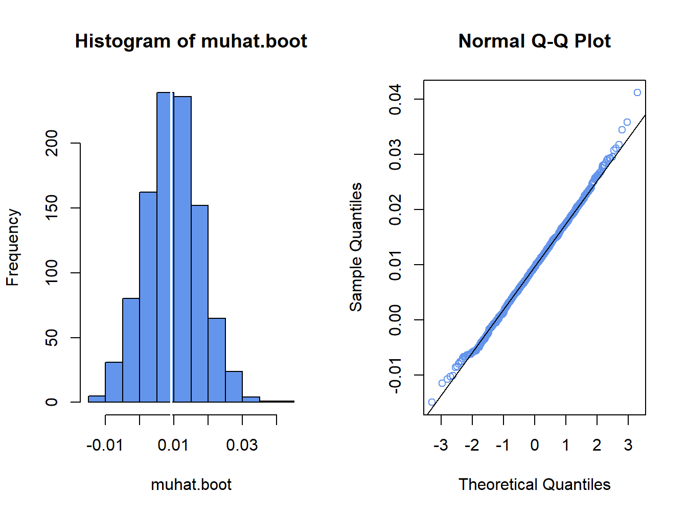
Figure 8.2: Histogram and normal QQ-plot of bootstrap estimates of \(\mu\) for Microsoft.
The distribution of the bootstrap estimates looks normal. As a result, the bootstrap 95% confidence interval for \(\mu\) has the form:
se.boot = sd(muhat.boot)
lower = muhatS + se.boot
upper = muhatS - se.boot
ans = cbind(muhatS, se.boot, lower, upper)
colnames(ans)=c("Estimate", "Std Error", "2.5%", "97.5%")
rownames(ans) = "mu"
ans
## Estimate Std Error 2.5% 97.5%
## mu 0.00915 0.00796 0.0171 0.0012\(\blacksquare\)
It is important to keep in mind that the bootstrap resampling algorithm draws random samples from the observed data. In the example above, the random number generator in R was initially set with set.seed(123). If the seed is set to a different integer, say 345, then the \(B=1,000\) bootstrap samples will be different and we will get different numerical results for the bootstrap bias and estimated standard error. How different these results will be depends on number of bootstrap samples \(B\) and the statistic \(\hat{\theta}\) being bootstrapped. Generally, the smaller is \(B\) the more variable the bootstraps results will be. It is good practice to repeat the bootstrap analysis with several different random number seeds to see how variable the results are. If the results vary considerably for different random number seeds then it is advised to increase the number of bootstrap simulations \(B\). It is common to use \(B=1,000\) for routine calculations, and \(B=10,000\) for final results.
8.6.4.2 R package boot
The R package boot implements a variety of bootstrapping
techniques including the basic non-parametric bootstrap described
above. The boot package was written to accompany the textbook Bootstrap Methods and Their Application by (Davison and Hinkley 1997).
The two main functions in boot are boot() and
boot.ci(), respectively. The boot() function implements
the bootstrap for a statistic computed from a user-supplied function.
The boot.ci() function computes bootstrap confidence intervals
given the output from the boot() function.
The arguments to boot() are:
## function (data, statistic, R, sim = "ordinary", stype = c("i",
##     "f", "w"), strata = rep(1, n), L = NULL, m = 0, weights = NULL,
##     ran.gen = function(d, p) d, mle = NULL, simple = FALSE, ...,
##     parallel = c("no", "multicore", "snow"), ncpus = getOption("boot.ncpus",
##         1L), cl = NULL)
## NULL
where data is a data object (typically a vector or matrix
but can be a time series object too), statistic is a use-specified
function to compute the statistic of interest, and R is the
number of bootstrap replications. The remaining arguments are not
important for the basic non-parametric bootstrap. The function assigned
to the argument statistic has to be written in a specific
form, which is illustrated in the next example. The boot()
function returns an object of class boot for which
there are print and plot methods.
The arguments to boot.ci() are
## function (boot.out, conf = 0.95, type = "all", index = 1L:min(2L,
##     length(boot.out$t0)), var.t0 = NULL, var.t = NULL, t0 = NULL,
##     t = NULL, L = NULL, h = function(t) t, hdot = function(t) rep(1,
##         length(t)), hinv = function(t) t, ...)
## NULL
where boot.out is an object of class boot,
conf specifies the confidence level, and type is
a subset from c("norm", "basic", "stud", "perc", "bca") indicating the type of confidence interval to compute.
The choices norm, perc, and “bca” compute the
normal confidence interval (8.16), the percentile
confidence interval (8.17), and the BCA confidence interval, respectively. The remaining arguments are not important for the computation of these
bootstrap confidence intervals.
To use the boot() function to implement the bootstrap for
\(\hat{\mu},\) a function must be specified to compute \(\hat{\mu}\)
for each bootstrap sample. The function must have two arguments: x
and idx. Here, x represents the original data and
idx represents the random integer index (created internally
by boot()) to subset x for each bootstrap sample.
For example, a function to be passed to boot() for \(\hat{\mu}\) is
mean.boot = function(x, idx) {
# arguments:
# x      data to be resampled
# idx    vector of scrambled indices created by boot() function
# value:
# ans   mean value computed using resampled data
    ans = mean(x[idx])
    ans
}
To implement the nonparametric bootstrap for \(\hat{\mu}\) with 999 samples use
## [1] "boot"## [1] "t0" "t" "R" "data" "seed" "statistic"
## [7] "sim" "call" "stype" "strata" "weights"The returned object muhat.boot is of class boot.
The component t0 is the sample estimate \(\hat{\mu}\), and
the component t is a \(999\times1\) matrix containing the bootstrap
estimates \(\{\hat{\mu}_{1}^{*},\ldots,\hat{\mu}_{999}^{*}\}\). The
print method shows the sample estimate, the bootstrap bias and the
bootstrap standard error:
##
## ORDINARY NONPARAMETRIC BOOTSTRAP
##
##
## Call:
## boot(data = msftRetS, statistic = mean.boot, R = 999)
##
##
## Bootstrap Statistics :
##     original   bias    std. error
## t1*  0.00915 0.000482     0.00758
These statistics can be computed directly from the components of muhat.boot
## [1] 0.009153 0.000482 0.007584A histogram and nornal QQ-plot of the bootstrap values, shown in Figure 8.3, can be created using the plot method
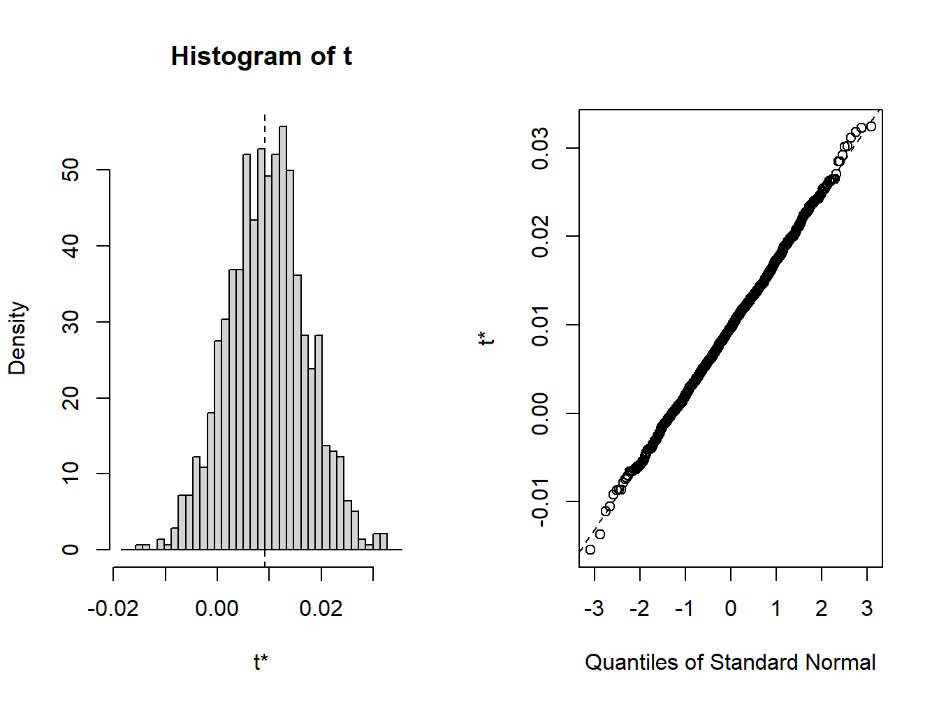
Figure 8.3: plot method for objects of class boot
Normal, percentile, and bias-adjusted (bca) percentile 95% confidence intervals can be computed using
## BOOTSTRAP CONFIDENCE INTERVAL CALCULATIONS
## Based on 999 bootstrap replicates
##
## CALL :
## boot.ci(boot.out = muhat.boot, conf = 0.95, type = c("norm",
##     "perc", "bca"))
##
## Intervals :
## Level      Normal             Percentile            BCa
## 95%   (-0.0062,  0.0235 )   (-0.0057,  0.0245 )   (-0.0062,  0.0239 )
## Calculations and Intervals on Original Scale
Because the bootstrap distribution looks normal, the normal, percentile, and bca confidence intervals are very similar.
The GWN model estimate \(\hat{\sigma}\) can be “bootstrapped” in a similar fashion. First, we write a function to compute \(\hat{\sigma}\) for each bootstrap sample
Then we call boot() with statistic=sd.boot
##
## ORDINARY NONPARAMETRIC BOOTSTRAP
##
##
## Call:
## boot(data = msftRetS, statistic = sd.boot, R = 999)
##
##
## Bootstrap Statistics :
##     original    bias    std. error
## t1*    0.101 -0.000783     0.00764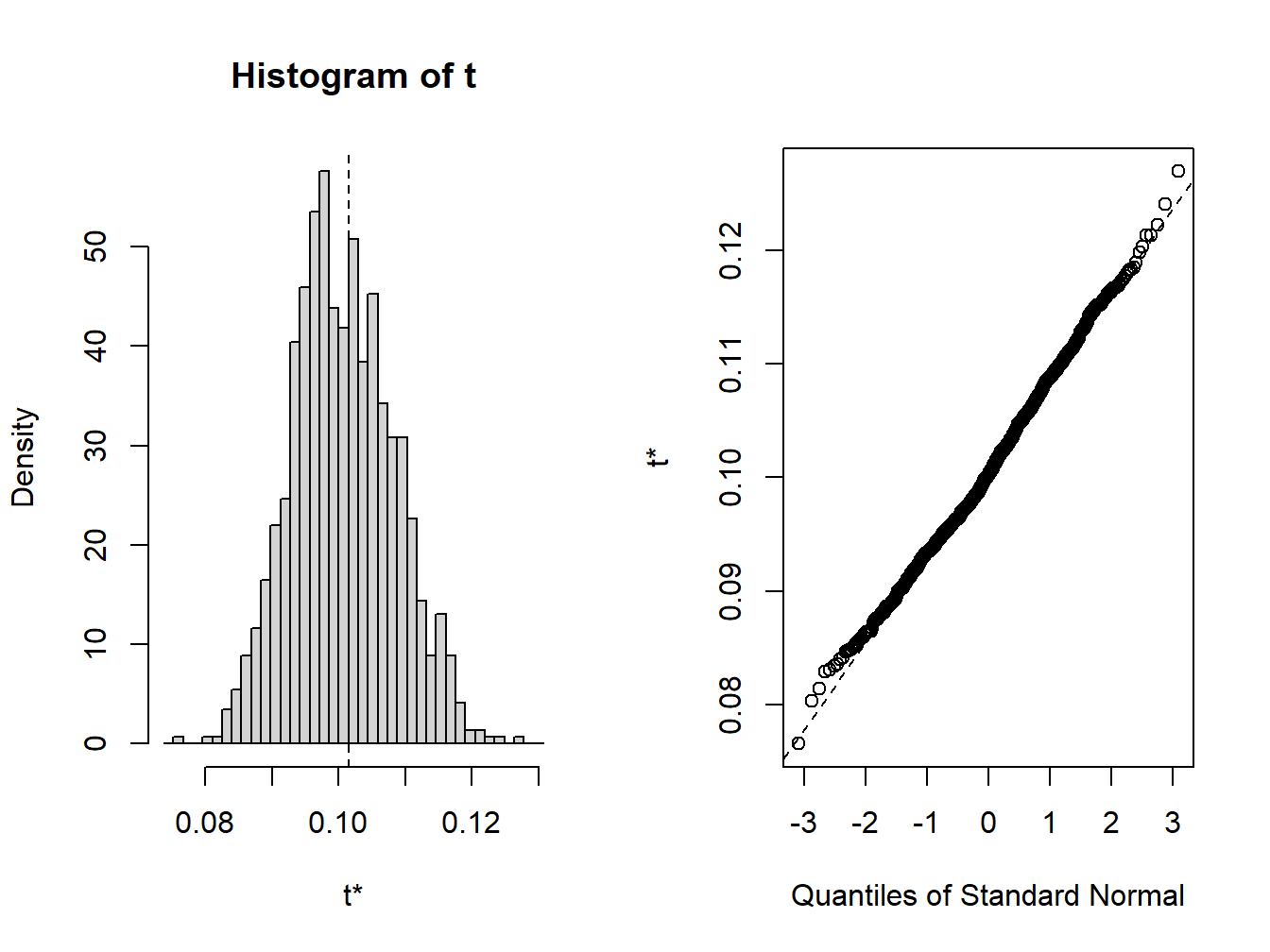
Figure 8.4: Bootstrap distribution for \(\hat{\sigma}\)
The bootstrap distribution, shown in Figure 8.4, looks a bit non-normal. The 95% confidences intervals are computed using
## BOOTSTRAP CONFIDENCE INTERVAL CALCULATIONS
## Based on 999 bootstrap replicates
##
## CALL :
## boot.ci(boot.out = sigmahat.boot, conf = 0.95, type = c("norm",
##     "perc", "bca"))
##
## Intervals :
## Level      Normal             Percentile            BCa
## 95%   ( 0.0873,  0.1173 )   ( 0.0864,  0.1162 )   ( 0.0892,  0.1200 )
## Calculations and Intervals on Original Scale
## Some BCa intervals may be unstable
We see that all of these intervals are quite similar.
\(\blacksquare\)
The real power of the bootstrap procedure comes when we apply it to
plug-in estimates of functions like (8.1)-(8.4) for which there
are no easy analytic formulas for estimating bias and standard errors. In this situation, the bootstrap procedure easily computes numerical estimates of the bias,
standard error, and 95% confidence interval. All we need is an R function for computing
the plug-in function estimate in a form suitable for boot(). The R functions for the example functions are:
f1.boot = function(x, idx, alpha=0.05) {
  q = mean(x[idx]) + sd(x[idx])*qnorm(alpha)
  q
}

f2.boot = function(x, idx, alpha=0.05, w0=100000) {
  q = mean(x[idx]) + sd(x[idx])*qnorm(alpha)
  VaR = -w0*q
  VaR
}

f3.boot = function(x, idx, alpha=0.05, w0=100000) {
    q = mean(x[idx]) + sd(x[idx])*qnorm(alpha)
    VaR = -(exp(q) - 1)*w0
    VaR
}

f4.boot = function(x, idx, r.f=0.0025) {
  SR = (mean(x[idx]) - r.f)/sd(x[idx])
  SR
}
The functions \(f_1\), \(f_2\), and \(f_3\) have the additional argument alpha
which specifies the tail probability for the quantile, and the functions \(f_2\), and \(f_3\) have the additional argument w0 for the initial wealth invested. The function \(f_4\) has the additional argument r.f for the risk-free rate.
To compute the nonparametric bootstrap for \(f_1\) with \(\alpha=0.05\) use:
##
## ORDINARY NONPARAMETRIC BOOTSTRAP
##
##
## Call:
## boot(data = msftRetS, statistic = f1.boot, R = 999)
##
##
## Bootstrap Statistics :
##     original  bias    std. error
## t1*   -0.158 0.00177      0.0124
Here, the bootstrap estimate of bias is small and the bootstrap estimated standard error is similar to the delta method and jackknife standard errors.
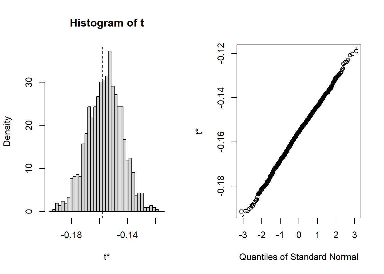
The bootstrap distribution looks normal, and the three methods for computing 95% confidence intervals are essentially the same:
## BOOTSTRAP CONFIDENCE INTERVAL CALCULATIONS
## Based on 999 bootstrap replicates
##
## CALL :
## boot.ci(boot.out = f1.bs, type = c("norm", "perc", "bca"))
##
## Intervals :
## Level      Normal             Percentile            BCa
## 95%   (-0.184, -0.135 )   (-0.181, -0.132 )   (-0.189, -0.138 )
## Calculations and Intervals on Original Scale
## Some BCa intervals may be unstable
To compute the nonparametric bootstrap for \(f_2\) with \(\alpha=0.05\) and \(W_0=\$100,000\) use:
##
## ORDINARY NONPARAMETRIC BOOTSTRAP
##
##
## Call:
## boot(data = msftRetS, statistic = f2.boot, R = 999)
##
##
## Bootstrap Statistics :
##     original  bias    std. error
## t1*    15780    -177        1244
The bootstrap estimate of bias is small and the bootstrap estimated standard error is similar to the delta method and jackknife standard errors.
The bootstrap distribution looks normal, and the three bootstrap 95% confidence intervals are all very similar:
## BOOTSTRAP CONFIDENCE INTERVAL CALCULATIONS
## Based on 999 bootstrap replicates
##
## CALL :
## boot.ci(boot.out = f2.bs, type = c("norm", "perc", "bca"))
##
## Intervals :
## Level Normal Percentile BCa
## 95% (13518, 18395 ) (13161, 18089 ) (13801, 18940 )
## Calculations and Intervals on Original Scale
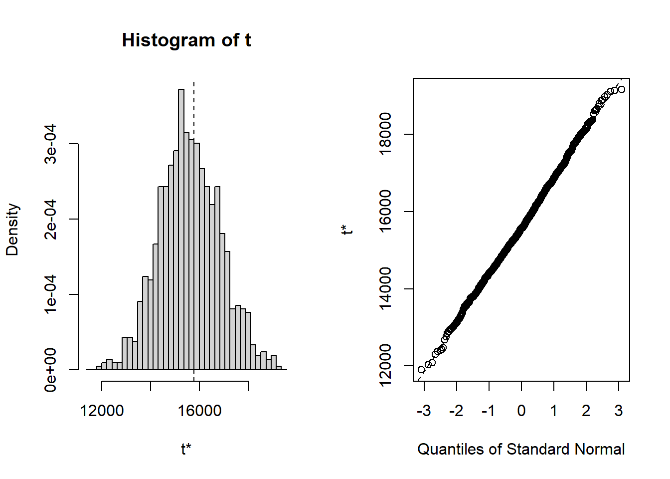
## Some BCa intervals may be unstableTo compute the nonparametric bootstrap for \(f_3\) with \(\alpha=0.05\) and \(W_0=\$100,000\) use:
##
## ORDINARY NONPARAMETRIC BOOTSTRAP
##
##
## Call:
## boot(data = msftRetC, statistic = f3.boot, R = 999)
##
##
## Bootstrap Statistics :
##     original  bias    std. error
## t1*    14846    -182        1223
The bias is small and the bootstrap estimated standard error is larger than the delta method standard error and is closer to the jackknife standard error.

The bootstrap distribution looks a little asymmetric and the BCA confidence interval is a bit different from the normal and percentile intervals:
## BOOTSTRAP CONFIDENCE INTERVAL CALCULATIONS
## Based on 999 bootstrap replicates
##
## CALL :
## boot.ci(boot.out = f3.bs, type = c("norm", "perc", "bca"))
##
## Intervals :
## Level      Normal             Percentile            BCa
## 95%   (12631, 17426 )   (12295, 17155 )   (12994, 18061 )
## Calculations and Intervals on Original Scale
## Some BCa intervals may be unstable
Finally, to compute the bootstrap for \(f_4\) with \(r_f = 0.0025\) use:
##
## ORDINARY NONPARAMETRIC BOOTSTRAP
##
##
## Call:
## boot(data = msftRetS, statistic = f4.boot, R = 999)
##
##
## Bootstrap Statistics :
##     original  bias    std. error
## t1*   0.0655 0.00391      0.0739
The bootstrap estimated bias is small and the standard error is similar to the delta method and the jackknife.
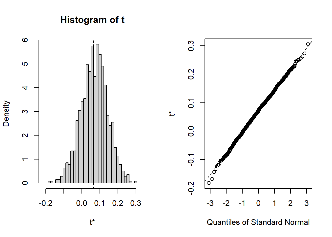
Here, the bootstrap distribution is slightly asymmetric.
## BOOTSTRAP CONFIDENCE INTERVAL CALCULATIONS
## Based on 999 bootstrap replicates
##
## CALL :
## boot.ci(boot.out = f4.bs, conf = 0.95, type = c("norm", "perc",
##     "bca"))
##
## Intervals :
## Level      Normal             Percentile            BCa
## 95%   (-0.0832,  0.2065 )   (-0.0821,  0.2132 )   (-0.0897,  0.2030 )
## Calculations and Intervals on Original Scale
Notice that the Percentile and BCA confidence intervals are a bit different from the normal approximation interval.
\(\blacksquare\)
8.6.5 Pros and cons of the nonparametric bootstrap
The nonparametric bootstrap is extremely useful and powerful statistical technique. The main advantages (pros) are:
General procedure to estimate bias and standard errors, and to compute confidence intervals, that does not rely on asymptotic distributions.
Can be used for scalar and vector estimates.
Under general conditions, bootstrap distributions of estimators converge to the asymptotic distribution of the estimators.
In certain situations, bootstrap results can be more accurate than analytic results computed from asymptotic distributions.
There are some things to watch out for when using the bootstrap (cons):
It be computational intensive but this is really not much of an issue with today’s fast computers.
With small \(B\), bootstrap results can vary substantially across simulations with different random number seeds.
There are situations where the bootstrap does not work. A leading case is when the bootstrap is applied to a function that can be become unbounded (e.g. a ratio of means when the denominator mean is close to zero). In these cases, a trimmed version of the bootstrap is recommended. See Hansen (2011) for a discussion of this issue.
You have to be careful applying the bootstrap to time series data. If there is serial correlation in the data then the nonparametric bootstrap may give poor results. There are versions of the bootstrap (e.g. the block bootstrap) that work with serial correlated data. For example, the tseries function
tsbootstrap()is designed to to work with serially correlated time series data.
References
Davison, A., and D. Hinkley. 1997. Bootstrap Methods and Their Application. Cambridge: Cambridge University Press.
We can also bootstrap data from multiple assets by defining \(r_t\) as a vector of asset returns.↩︎
The bootstrap percentile-t confidence interval is another bias and skewness adjusted confidence interval.↩︎
We use
set.seed(123)to initialize the random number generator in R and allow for reproducible results.↩︎