12.3 Determining Mean-Variance Efficient Portfolios Using Matrix Algebra
The investment opportunity set is the set of portfolio expected return, \(\mu_{p}\), and portfolio standard deviation, \(\sigma_{p}\), values for all possible portfolios whose weights sum to one. As in the two risky asset case, this set can be described in a graph with \(\mu_{p}\) on the vertical axis and \(\sigma_{p}\) on the horizontal axis. With two assets, the investment opportunity set in (\(\mu_{p},\sigma_{p}\))-space lies on a curve (one side of a hyperbola). With three or more assets, the investment opportunity set in (\(\mu_{p},\sigma_{p}\))-space is described by set of values whose general shape is complicated and depends crucially on the covariance terms \(\sigma_{ij}\).80 However, we do not have to fully characterize the entire investment opportunity set. If we assume that investors choose portfolios to maximize expected return subject to a target level of risk, or, equivalently, to minimize risk subject to a target expected return, then we can simplify the asset allocation problem by only concentrating on the set of efficient portfolios. These portfolios lie on the boundary of the investment opportunity set above the global minimum variance portfolio. This is the framework originally developed by Harry Markowitz, the father of portfolio theory and winner of the Nobel Prize in economics.
Following Markowitz, we assume that investors wish to find portfolios that have the best expected return-risk trade-off. We can characterize these efficient portfolios in two equivalent ways. In the first way, investors seek to find portfolios that maximize portfolio expected return for a given level of risk as measured by portfolio variance. Let \(\sigma_{p,0}^{2}\) denote a target level of risk. Then the constrained maximization problem to find an efficient portfolio is: \[\begin{align} \max_{\mathbf{x}}\mu_{p} & =\mathbf{x}^{\prime}\mu \tag{12.9}\\ \textrm{ s.t. } \sigma_{p}^{2} & =\mathbf{x}^{\prime}\Sigma \mathbf{x}=\sigma_{p,0}^{2}\textrm{ and }\mathbf{x}^{\prime}\mathbf{1}=1.\nonumber \end{align}\] The investor’s problem of maximizing portfolio expected return subject to a target level of risk has an equivalent dual representation in which the investor minimizes the risk of the portfolio (as measured by portfolio variance) subject to a target expected return level. Let \(\mu_{p,0}\) denote a target expected return level. Then the dual problem is the constrained minimization problem:81 \[\begin{align} \min_{\mathbf{x}}~\sigma_{p,x}^{2} & =\mathbf{x}^{\prime}\Sigma \mathbf{x} \tag{12.10}\\ \textrm{ s.t. } \mu_{p} & =\mathbf{x}^{\prime}\mu=\mu_{p,0}\mathbf{,}\textrm{ and }\mathbf{x}^{\prime}\mathbf{1}=1.\nonumber \end{align}\] To find efficient portfolios of risky assets in practice, the dual problem (12.10) is most often solved. This is partially due to computational conveniences and partly due to investors being more willing to specify target expected returns rather than target risk levels. The efficient portfolio frontier is a graph of \(\mu_{p}\) versus \(\sigma_{p}\) values for the set of efficient portfolios generated by solving (12.10) for all possible target expected return levels \(\mu_{p,0}\) above the expected return on the global minimum variance portfolio. Just as in the two asset case, the resulting efficient frontier will resemble one side of an hyperbola and is often called the “Markowitz bullet”. This frontier is illustrated in Figure 12.3 as the boundary of the set generated by random portfolios above the global minimum variance portfolio.
To solve the constrained minimization problem (12.10), first form the Lagrangian function: \[ L(x,\lambda_{1},\lambda_{2})=\mathbf{x}^{\prime}\Sigma \mathbf{x}+\lambda_{1}(\mathbf{x}^{\prime}\mathbf{\mu-}\mu_{p,0})+\lambda_{2}(\mathbf{x}^{\prime}\mathbf{1}-1). \] Because there are two constraints (\(\mathbf{x}^{\prime}\mu=\mu_{p,0}\) and \(\mathbf{x}^{\prime}\mathbf{1}=1)\) there are two Lagrange multipliers \(\lambda_{1}\) and \(\lambda_{2}\). The FOCs for a minimum are the linear equations: \[\begin{align} \frac{\partial L(\mathbf{x},\lambda_{1},\lambda_{2})}{\partial\mathbf{x}} & =2\Sigma \mathbf{x}+\lambda_{1}\mu+\lambda_{2}\mathbf{1}=\mathbf{0,}\tag{12.11}\\ \frac{\partial L(\mathbf{x},\lambda_{1},\lambda_{2})}{\partial\lambda_{1}} & =\mathbf{x}^{\prime}\mu-\mu_{p,0}=0,\tag{12.12}\\ \frac{\partial L(\mathbf{x},\lambda_{1},\lambda_{2})}{\partial\lambda_{2}} & =\mathbf{x}^{\prime}\mathbf{1}-1=0.\tag{12.13} \end{align}\] These FOCs consist of \(N+2\) linear equations in \(N+2\) unknowns (\(\mathbf{x},\,\lambda_{1},\,\lambda_{2})\). We can represent the system of linear equations using matrix algebra as: \[ \left(\begin{array}{ccc} 2\Sigma & \mu & \mathbf{1}\\ \mu^{\prime} & 0 & 0\\ \mathbf{1}^{\prime} & 0 & 0 \end{array}\right)\left(\begin{array}{c} \mathbf{x}\\ \lambda_{1}\\ \lambda_{2} \end{array}\right)=\left(\begin{array}{c} \mathbf{0}\\ \mu_{p,0}\\ 1 \end{array}\right), \] which is of the form \(\mathbf{Az}_{x}\mathbf{=b}_{0}\), where \[ \mathbf{A}=\left(\begin{array}{ccc} 2\Sigma & \mu & \mathbf{1}\\ \mu^{\prime} & 0 & 0\\ \mathbf{1}^{\prime} & 0 & 0 \end{array}\right),~\mathbf{z}_{x}=\left(\begin{array}{c} \mathbf{x}\\ \lambda_{1}\\ \lambda_{2} \end{array}\right)\textrm{ and }\mathbf{b}_{0}=\left(\begin{array}{c} \mathbf{0}\\ \mu_{p,0}\\ 1 \end{array}\right). \] The solution for \(\mathbf{z}_{x}\) is then: \[\begin{equation} \mathbf{z}_{x}=\mathbf{A}^{-1}\mathbf{b}_{0}.\tag{12.14} \end{equation}\] The first \(N\) elements of \(\mathbf{z}_{x}\) are the portfolio weights \(\mathbf{x}\) for the minimum variance portfolio with expected return \(\mu_{p,x}=\mu_{p,0}\). If \(\mu_{p,0}\) is greater than or equal to the expected return on the global minimum variance portfolio, then \(\mathbf{x}\) is an efficient (frontier) portfolio. Otherwise, it is an inefficient (frontier) portfolio.
Using the data in Table 12.1, consider finding a minimum variance portfolio with the same expected return as Microsoft. This will be an efficient portfolio because \(\mu_{\textrm{msft}}=0.043>\mu_{p,m}=0.025\). Call this portfolio \(\mathbf{x}=(x_{\textrm{msft}},x_{\textrm{nord}},x_{\textrm{sbux}})^{\prime}\). That is, consider solving (12.10) with target expected return \(\mu_{p,0}=\mu_{\textrm{msft}}=0.043\) using (12.14). The R calculations to create the matrix \(\mathbf{A}_{x}\) and the vectors \(\mathbf{z}_{x}\) and \(\mathbf{b}_{\textrm{msft}}\) are:
top.mat = cbind(2*sigma.mat, mu.vec, rep(1, 3))
mid.vec = c(mu.vec, 0, 0)
bot.vec = c(rep(1, 3), 0, 0)
Ax.mat = rbind(top.mat, mid.vec, bot.vec)
bmsft.vec = c(rep(0, 3), mu.vec["MSFT"], 1)
and the R code to solve for \(\mathbf{x}\) using (12.14) is:
##    MSFT    NORD    SBUX
##  0.8275 -0.0907  0.2633
The efficient portfolio with the same expected return as Microsoft has portfolio weights \(x_{\textrm{msft}}=0.8275\), \(x_{\textrm{nord}}=-0.0907\) and \(x_{\textrm{sbux}}=0.2633\), and is given by the vector \(\mathbf{x}=(0.8275,-0.0907,0.2633)^{\prime}.\) The expected return on this portfolio, \(\mu_{p,x}=\mathbf{x}^{\prime}\mu\), is equal to the target return \(\mu_{\textrm{msft}}\):
## [1] 0.0427The portfolio variance, \(\sigma_{p,x}^{2}=\mathbf{x}^{\prime}\Sigma \mathbf{x}\), and standard deviation, \(\sigma_{p,x}\), are:
## [1] 0.0084 0.0917and are smaller than the corresponding values for Microsoft (see Table 12.1). This efficient portfolio is labeled “E1” in Figure 12.5.
\(\blacksquare\)
To find a minimum variance portfolio \(\mathbf{y}=(y_{\textrm{msft}},y_{\textrm{nord}},y_{\textrm{sbux}})^{\prime}\) with the same expected return as Starbucks we use (12.14) with \(\mathbf{b}_{\textrm{sbux}}=(\mathbf{0},\mu_{\textrm{sbux}},1)^{\prime}\):
bsbux.vec = c(rep(0, 3), mu.vec["SBUX"], 1)
z.mat = solve(Ax.mat)%*%bsbux.vec
y.vec = z.mat[1:3,]
y.vec
## MSFT NORD SBUX
## 0.519 0.273 0.207The portfolio \(\mathbf{y}=(0.519,0.273,0.207)^{\prime}\) is an efficient portfolio on the outer boundary because \(\mu_{\textrm{sbux}}=0.0285>\mu_{p,m}=0.0249\). The portfolio expected return and standard deviation are:
mu.py = as.numeric(crossprod(y.vec, mu.vec))
sig2.py = as.numeric(t(y.vec)%*%sigma.mat%*%y.vec)
sig.py = sqrt(sig2.py)
c(mu.py,sig.py)
## [1] 0.0285 0.0736This efficient portfolio is labeled “E2” in Figure 12.5. It has the same expected return as SBUX but a smaller standard deviation.
The covariance and correlation values between the portfolio returns \(R_{p,x}=\mathbf{x}^{\prime}\mathbf{R}\) and \(R_{p,y}=\mathbf{y}^{\prime}\mathbf{R}\) are given by:
sigma.xy = as.numeric(t(x.vec)%*%sigma.mat%*%y.vec)
rho.xy = sigma.xy/(sig.px*sig.py)
c(sigma.xy, rho.xy)
## [1] 0.00591 0.87722This covariance will be used later on when constructing the entire frontier of efficient portfolios.
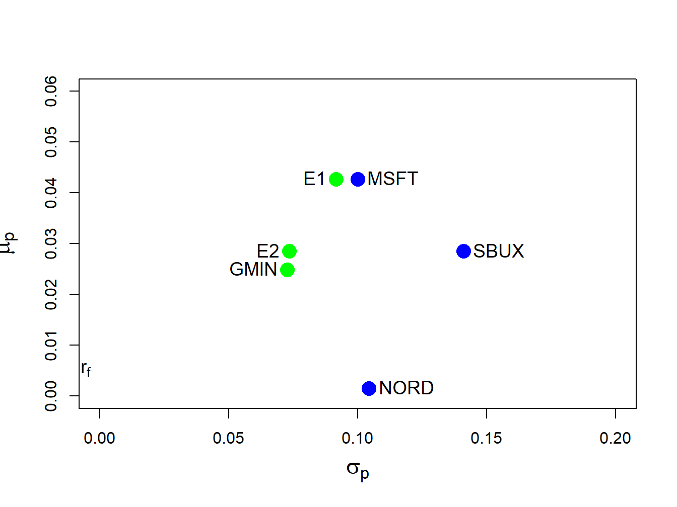
Figure 12.5: Minimum variance efficient portfolios from example data. Portfolio “E1” has the same expected return as Microsoft, and portfolio “E2” has the same expected returns as Starbucks.
12.3.1 Alternative derivation of an efficient portfolio
The equation (12.14) does not give an explicit solution for the minimum variance portfolio \(\mathbf{x}\). As with the global minimum variance portfolio (12.8), an explicit solution for \(\mathbf{x}\) can also be found. Consider the first order conditions (12.11)-(12.13) from the optimization problem (12.10). First, use (12.11) to solve for the \(N\times1\) vector \(\mathbf{x}\): \[\begin{equation} \mathbf{x}=-\frac{1}{2}\lambda_{1}\Sigma^{-1}\mu-\frac{1}{2}\lambda_{2}\Sigma^{-1}\mathbf{1}.\tag{12.15} \end{equation}\] Define the \(N\times2\) matrix \(\mathbf{M}=[\mu\) \(\vdots\) \(\mathbf{1}]\) and the \(2\times1\) vector \(\lambda=(\lambda_{1},\lambda_{2})^{\prime}\). Then we can rewrite (12.15) in matrix form as: \[\begin{equation} \mathbf{x}=-\frac{1}{2}\Sigma^{-1}\mathbf{M}\lambda.\tag{12.16} \end{equation}\] Next, to find the values for \(\lambda_{1}\) and \(\lambda_{2}\), pre-multiply (12.15) by \(\mu^{\prime}\) and use (12.12) to give: \[\begin{equation} \mu_{0}=\mu^{\prime}\mathbf{x}=-\frac{1}{2}\lambda_{1}\mu^{\prime}\Sigma^{-1}\mu-\frac{1}{2}\lambda_{2}\mu^{\prime}\Sigma^{-1}\mathbf{1}.\tag{12.17} \end{equation}\] Similarly, pre-multiply (12.15) by \(\mathbf{1}^{\prime}\) and use (12.13) to give: \[\begin{equation} 1=\mathbf{1}^{\prime}\mathbf{x}=-\frac{1}{2}\lambda_{1}\mathbf{1}^{\prime}\Sigma^{-1}\mu-\frac{1}{2}\lambda_{2}\mathbf{1}^{\prime}\Sigma^{-1}\mathbf{1}.\tag{12.18} \end{equation}\] Now, we have two linear equations (12.17) and (12.18) involving \(\lambda_{1}\) and \(\lambda_{2}\) which we can write in matrix notation as: \[\begin{equation} -\frac{1}{2}\left(\begin{array}{cc} \mu^{\prime}\Sigma^{-1}\mu & \mu^{\prime}\Sigma^{-1}\mathbf{1}\\ \mu^{\prime}\Sigma^{-1}\mathbf{1} & \mathbf{1}^{\prime}\Sigma^{-1}\mathbf{1} \end{array}\right)\left(\begin{array}{c} \lambda_{1}\\ \lambda_{2} \end{array}\right)=\left(\begin{array}{c} \mu_{0}\\ 1 \end{array}\right).\tag{12.19} \end{equation}\] Define, \[\begin{align*} \left(\begin{array}{cc} \mu^{\prime}\Sigma^{-1}\mu & \mu^{\prime}\Sigma^{-1}\mathbf{1}\\ \mu^{\prime}\Sigma^{-1}\mathbf{1} & \mathbf{1}^{\prime}\Sigma^{-1}\mathbf{1} \end{array}\right) & =\mathbf{M}^{\prime}\Sigma^{-1}\mathbf{M=B},\\ \tilde{\mu}_{0} & =\left(\begin{array}{c} \mu_{0}\\ 1 \end{array}\right), \end{align*}\] so that we can rewrite (12.19) as, \[ -\frac{1}{2}\mathbf{B}\lambda=\tilde{\mu}_{0}. \] Provided \(\mathbf{B}\) is invertible, the solution for \(\lambda=(\lambda_{1},\lambda_{2})^{\prime}\) is \[\begin{equation} \lambda=-2\mathbf{B}^{-1}\tilde{\mu}_{0}.\tag{12.20} \end{equation}\] Substituting (12.20) back into (12.16) gives an explicit expression for the efficient portfolio weight vector \(\mathbf{x}:\) \[\begin{equation} \mathbf{x}=-\frac{1}{2}\Sigma^{-1}\mathbf{M}\lambda=-\frac{1}{2}\Sigma^{-1}\mathbf{M}\left(-2\mathbf{B}^{-1}\tilde{\mu}_{0}\right)=\Sigma^{-1}\mathbf{MB}^{-1}\tilde{\mu}_{0}.\tag{12.21} \end{equation}\]
The R code to compute the efficient portfolio with the same expected return as Microsoft using (12.21) is:
M.mat = cbind(mu.vec, one.vec)
B.mat = t(M.mat)%*%solve(sigma.mat)%*%M.mat
mu.tilde.msft = c(mu.vec["MSFT"], 1)
x.vec.2 = solve(sigma.mat)%*%M.mat%*%solve(B.mat)%*%mu.tilde.msft
t(x.vec.2)
## MSFT NORD SBUX
## [1,] 0.827 -0.0907 0.263\(\blacksquare\)