7.6 Using Monte Carlo Simulation to Understand the Statistical Properties of Estimators

Let \(R_{t}\) be the return on a single asset described by the GWN model, let \(\theta\) denote some characteristic (parameter) of the GWN model we are interested in estimating, and let \(\hat{\theta}\) denote an estimator for \(\theta\) based on a sample of size \(T\). The exact meaning of estimator bias, \(\mathrm{bias}(\hat{\theta},\theta)\), the interpretation of \(\mathrm{se}(\hat{\theta})\) as a measure of precision, the sampling distribution \(f(\hat{\theta})\), and the interpretation of the coverage probability of a confidence interval for \(\theta\), can all be a bit hard to grasp at first. If \(\mathrm{bias}(\hat{\theta},\theta)=0\) so that \(E[\hat{\theta}]=\theta\) then over an infinite number of repeated samples of \(\{R_{it}\}_{t=1}^{T}\) the average of the \(\hat{\theta}\) values computed over the infinite samples is equal to the true value \(\theta\). The value of \(\mathrm{se}(\hat{\theta})\) represents the standard deviation of these \(\hat{\theta}\) values. The sampling distribution \(f(\hat{\theta})\) is the smoothed histogram of these \(\hat{\theta}\) values. And the 95% confidence intervals for \(\theta\) will actually contain \(\theta\) in 95% of the samples. We can think of these hypothetical samples as different Monte Carlo simulations of the GWN model. In this way we can approximate the computations involved in evaluating \(E[\hat{\theta}]\), \(\mathrm{se}(\hat{\theta})\), \(f(\hat{\theta})\), and the coverage probability of a confidence interval using a large, but finite, number of Monte Carlo simulations.

7.6.1 Evaluating the Statistical Properties of \(\hat{\mu}\) Using Monte Carlo Simulation

Consider the GWN model: \[\begin{align} R_{t} & =0.05+\varepsilon_{t},t=1,\ldots,100\tag{7.41}\\ & \varepsilon_{t}\sim\mathrm{GWN}(0,(0.10)^{2}).\nonumber \end{align}\] Here, the true parameter values are \(\mu=0.05\) and \(\sigma=0.10\). Using Monte Carlo simulation, we can simulate \(N=1000\) different samples of size \(T=100\) from (7.41) giving the sample realizations \(\{r_{t}^{j}\}_{t=1}^{100}\) for \(j=1,\ldots,1000\). The R code to perform the Monte Carlo simulation is:

mu = 0.05
sigma = 0.10
n.obs = 100
n.sim = 1000
set.seed(111)
sim.means = rep(0,n.sim)
mu.lower = rep(0,n.sim)
mu.upper = rep(0,n.sim)
qt.975 = qt(0.975, n.obs-1)
for (sim in 1:n.sim) {
    sim.ret = rnorm(n.obs,mean=mu,sd=sigma)
    sim.means[sim] = mean(sim.ret)
    se.muhat = sd(sim.ret)/sqrt(n.obs)
    mu.lower[sim] = sim.means[sim]-qt.975*se.muhat
    mu.upper[sim] = sim.means[sim]+qt.975*se.muhat
}

The first 10 of these simulated samples are illustrated in Figure 7.5. Notice that there is considerable variation in the appearance of the simulated samples, but that all of the simulated samples fluctuate about the true mean value of \(\mu=0.05\) and have a typical deviation from the mean of about \(0.10\).

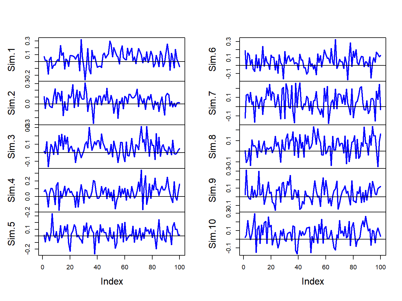
Figure 7.5: Ten simulated samples of size \(T=100\) from the GWN model \(R_{t}=0.05+\varepsilon_{t}\), \(\varepsilon_{t}\sim iid~N(0,(0.10)^{2})\).

For each of the \(1000\) simulated samples we can estimate \(\hat{\mu}\) giving \(1000\) mean estimates \(\{\hat{\mu}^{1},\ldots,\hat{\mu}^{1000}\}\). A histogram of these \(1000\) mean values is illustrated in Figure 7.6.

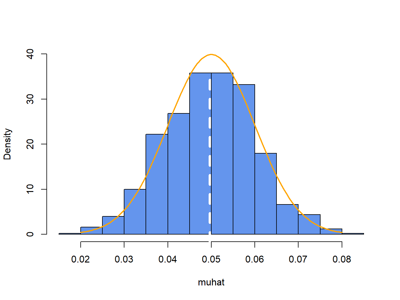
Figure 7.6: Distribution of \(\hat{\mu}\) computed from \(1000\) Monte Carlo simulations from the GWN model (7.41). White dashed line is the average of the \(\mu\) values, and orange curve is the true \(f(\hat{\mu})\).

The histogram of the estimated means, \(\hat{\mu}^{j}\), can be thought of as an estimate of the underlying pdf, \(f(\hat{\mu})\), of the estimator \(\hat{\mu}\) which we know from (7.29) is a normal pdf centered at \(E[\hat{\mu}]=\mu=0.05\) with \(\mathrm{se}(\hat{\mu}_{i})=0.10/\sqrt{100}=0.01\). This normal curve (solid orange line) is superimposed on the histogram in Figure 7.6. Notice that the center of the histogram (white dashed vertical line) is very close to the true mean value \(\mu=0.05\). That is, on average over the \(1000\) Monte Carlo samples the value of \(\hat{\mu}\) is about 0.05. In some samples, the estimate is too big and in some samples the estimate is too small but on average the estimate is correct. In fact, the average value of \(\{\hat{\mu}^{1},\ldots,\hat{\mu}^{1000}\}\) from the \(1000\) simulated samples is: \[ \overline{\hat{\mu}}=\frac{1}{1000}\sum_{j=1}^{1000}\hat{\mu}^{j}=0.0497, \] which is very close to the true value \(0.05\). If the number of simulated samples is allowed to go to infinity then the sample average \(\overline{\hat{\mu}}\) will be exactly equal to \(\mu=0.05\): \[ \lim_{N\rightarrow\infty}\frac{1}{N}\sum_{j=1}^{N}\hat{\mu}^{j}=E[\hat{\mu}]=\mu=0.05. \]

The typical size of the spread about the center of the histogram represents \(\mathrm{se}(\hat{\mu}_{i})\) and gives an indication of the precision of \(\hat{\mu}_{i}\). The value of \(\mathrm{se}(\hat{\mu}_{i})\) may be approximated by computing the sample standard deviation of the \(1000\) \(\hat{\mu}^{j}\) values: \[ \hat{\sigma}_{\hat{\mu}}=\sqrt{\frac{1}{999}\sum_{j=1}^{1000}(\hat{\mu}^{j}-0.04969)^{2}}=0.0104. \] Notice that this value is very close to the exact standard error: \(\mathrm{se}(\hat{\mu}_{i})=0.10/\sqrt{100}=0.01\). If the number of simulated sample goes to infinity then: \[ \lim_{N\rightarrow\infty}\sqrt{\frac{1}{N-1}\sum_{j=1}^{N}(\hat{\mu}^{j}-\overline{\hat{\mu}})^{2}}=\mathrm{se}(\hat{\mu}_{i})=0.01. \]

The coverage probability of the 95% confidence interval for \(\mu\) can also be illustrated using Monte Carlo simulation. For each simulation \(j\), the interval \(\hat{\mu}^j \pm t_{100}(0.975)\times\widehat{\mathrm{se}}(\hat{\mu}^{j})\) is computed. The coverage probability is approximated by the fraction of intervals that contain (cover) the true \(\mu=0.05\). For the 1000 simulated samples, this fraction turns out to be 0.931. As the number of simulations goes to infinity, the Monte Carlo coverage probability will be equal to 0.95.

Here are the R results to support the above calculations. The mean and standard deviation of \(\{\hat{\mu}^{1},\ldots,\hat{\mu}^{1000}\}\) are:

ans = c(mean(sim.means), sd(sim.means))
names(ans) = c("Mu", "Sigma")
ans

##     Mu  Sigma 
## 0.0497 0.0104

To evaluate the coverage probability of the 95% confidence intervals, we count the number of times each interval actually contains the true value of \(\mu\):

in.interval = mu >= mu.lower & mu <= mu.upper
sum(in.interval)/n.sim

## [1] 0.931

7.6.2 Evaluating the Statistical Properties of \(\hat{\sigma}_{i}^{2}\) and \(\hat{\sigma}_{i}\) Using Monte Carlo simulation

We can evaluate the statistical properties of \(\hat{\sigma}_{i}^{2}\) and \(\hat{\sigma}_{i}\) by Monte Carlo simulation in the same way that we evaluated the statistical properties of \(\hat{\mu}_{i}\). We use the simulation model (7.41) and \(N=1000\) simulated samples of size \(T=100\) to compute the estimates \(\{\left(\hat{\sigma}^{2}\right)^{1},\ldots,\left(\hat{\sigma}^{2}\right)^{1000}\}\) and \(\{\hat{\sigma}^{1},\ldots,\hat{\sigma}^{1000}\}\). The R code for the simulation loop is:

mu = 0.05
sigma = 0.10
n.obs = 100
n.sim = 1000
set.seed(111)
sim.sigma2 = rep(0,n.sim)
sigma2.lower = rep(0,n.sim)
sigma2.upper = rep(0,n.sim)
sim.sigma = rep(0,n.sim)
sigma.lower = rep(0,n.sim)
sigma.upper = rep(0,n.sim)
for (sim in 1:n.sim) {
    sim.ret = rnorm(n.obs,mean=mu,sd=sigma)
    sim.sigma2[sim] = var(sim.ret)
    sim.sigma[sim] = sqrt(sim.sigma2[sim])
    sigma2.lower[sim] = sim.sigma2[sim] - 2*sim.sigma2[sim]/sqrt(n.obs/2)
    sigma2.upper[sim] = sim.sigma2[sim] + 2*sim.sigma2[sim]/sqrt(n.obs/2)
    sigma.lower[sim] = sim.sigma[sim] - 2*sim.sigma[sim]/sqrt(n.obs*2)
    sigma.upper[sim] = sim.sigma[sim] + 2*sim.sigma[sim]/sqrt(n.obs*2)
}

The histograms of these values, with the asymptotic normal distributions overlayed, are displayed in Figure 7.7. The histogram for the \(\hat{\sigma}^{2}\) values is bell-shaped and slightly right skewed but is centered very close to \(\sigma^{2}=0.010\). The histogram for the \(\hat{\sigma}\) values is more symmetric and is centered near \(\sigma=0.10\).

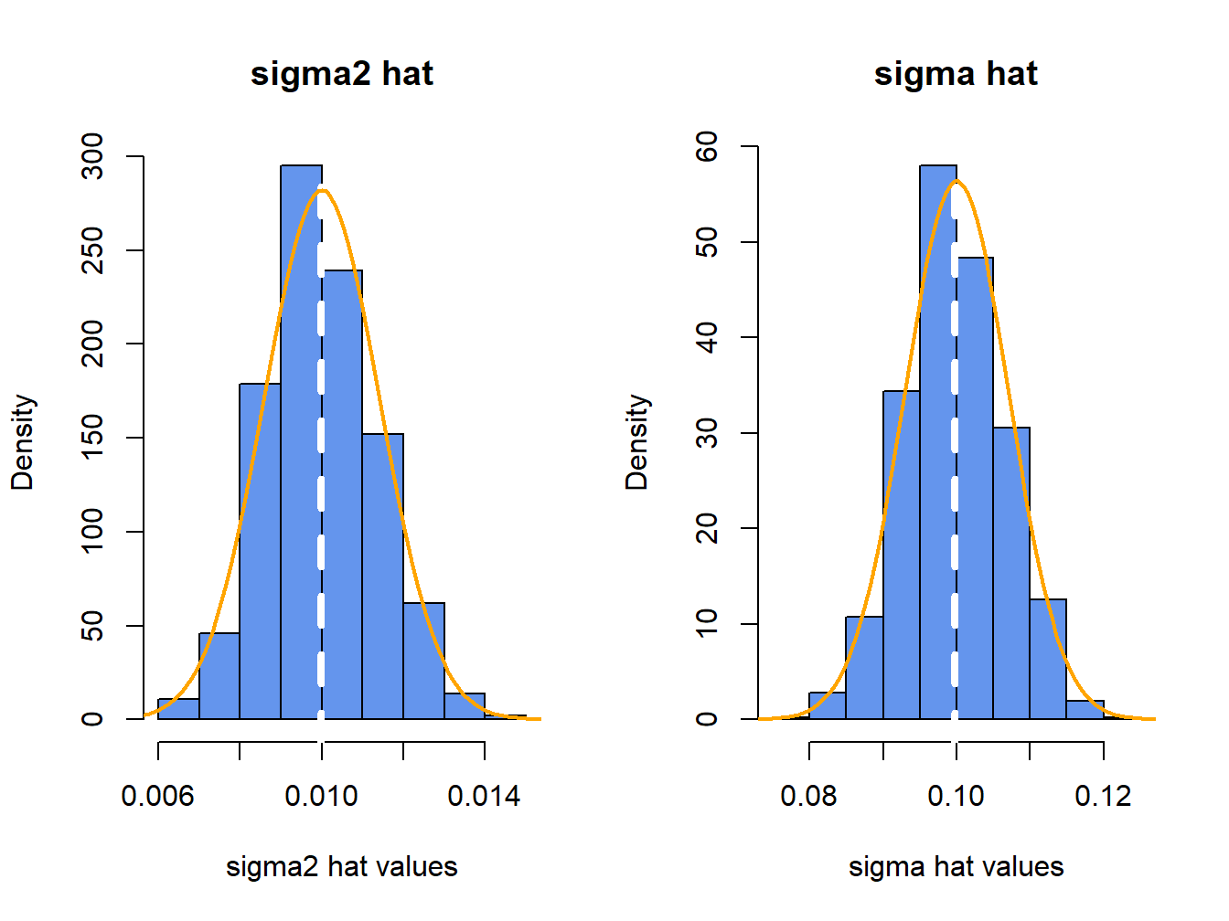
Figure 7.7: Histograms of \(\hat{\sigma}^{2}\) and \(\hat{\sigma}\) computed from \(N=1000\) Monte Carlo samples from GWN model.

The average values of \(\hat{\sigma}^{2}\) and \(\hat{\sigma}\) from the \(1000\) simulations are: \[\begin{align*} \overline{\hat{\sigma}^{2}} & =\frac{1}{1000}\sum_{j=1}^{1000}\left(\hat{\sigma}^{2}\right)^{j}=0.00999,\\ \overline{\hat{\sigma}} & =\frac{1}{1000}\sum_{j=1}^{1000}\hat{\sigma}^{j}=0.0997. \end{align*}\] The Monte Carlo estimate of the bias for \(\hat{\sigma}^{2}\) is \(0.00999-0.01=-0.0000\), and the estimate of bias for \(\hat{\sigma}\) is \(0.0997-0.010=-0.0003\). This confirms that \(\hat{\sigma}^{2}\) is unbiased and that the bias in \(\hat{\sigma}\) is extremely small. If the number of simulated samples, \(N\), goes to infinity then \(\overline{\hat{\sigma}^{2}}\rightarrow E[\hat{\sigma}^{2}]=\sigma^{2}=0.01\), and \(\overline{\hat{\sigma}}\rightarrow E[\hat{\sigma}]=\sigma+\mathrm{bias}(\hat{\sigma},\sigma)\).

The sample standard deviation values of the Monte Carlo estimates of \(\sigma^{2}\) and \(\sigma\) give approximations to \(\mathrm{se}(\hat{\sigma}^{2})\) and \(\mathrm{se}(\hat{\sigma})\): \[\begin{align*} \hat{\sigma}_{\hat{\sigma}^{2}} & =\sqrt{\frac{1}{999}\sum_{j=1}^{1000}((\hat{\sigma}^{2})^{j}-0.00999)^{2}}=0.00135,\\ \hat{\sigma}_{\hat{\sigma}} & =\sqrt{\frac{1}{999}\sum_{j=1}^{1000}(\hat{\sigma}^{j}-0.0997)^{2}}=0.00676. \end{align*}\] The approximate values for \(\mathrm{se}(\hat{\sigma}^{2})\) and \(\mathrm{se}(\hat{\sigma})\) based on the CLT are: \[\begin{align*} \mathrm{se}(\hat{\sigma}^{2}) & =\frac{(0.10)^{2}}{\sqrt{100/2}}=0.00141,\\ \mathrm{se}(\hat{\sigma}^{2}) & =\frac{0.10}{\sqrt{2\times100}}=0.00707. \end{align*}\] Notice that the Monte Carlo estimates of \(\mathrm{se}(\hat{\sigma}^{2})\) and \(\mathrm{se}(\hat{\sigma})\) are a bit different from the CLT based estimates. The reason is that the CLT based estimates are approximations that hold when the sample size \(T\) is large. Because \(T=100\) is not too large, the Monte Carlo estimates of s\(\mathrm{e}(\hat{\sigma}^{2})\) and \(\mathrm{se}(\hat{\sigma})\) are likely more accurate (and will be more accurate if the number of simulations is larger).

For each simulation \(j\), the approximate 95% confidence intervals \((\hat{\sigma}^{2})^{j}\pm2\times\widehat{\mathrm{se}}((\hat{\sigma}^{2})^{j})\) and \(\hat{\sigma}^{j}\pm2\times\widehat{\mathrm{se}}(\hat{\sigma}^{j})\) are computed. The coverage probabilities of these intervals is approximated by the fractions of intervals that contain (cover) the true values \(\sigma^{2}=0.01\) and \(\sigma=0.10\) respectively. For the 1000 simulated samples, these fractions turn out to be 0.951 and 0.963, respectively. As the number of simulations and the sample size go to infinity, the Monte Carlo coverage probability will be equal to 0.95.

Here is the R code to support the above calculation. The mean values and biases of the estimates are:

ans = rbind(c(sigma^2,mean(sim.sigma2),mean(sim.sigma2) - sigma^2),
            c(sigma, mean(sim.sigma), mean(sim.sigma) - sigma))
colnames(ans) = c("True Value", "Mean", "Bias")
rownames(ans) = c("Variance", "Volatility")
round(ans, digits=5)

##            True Value    Mean     Bias
## Variance         0.01 0.00999 -0.00001
## Volatility       0.10 0.09972 -0.00028

The Monte Carlo and analytic standard error estimates are:

ans = rbind(c(sd(sim.sigma2),sigma^2/sqrt(n.obs/2)),
            c(sd(sim.sigma), sigma/sqrt(2*n.obs)))
colnames(ans) = c("MC Std Error", "Analytic Std Error")
rownames(ans) = c("Variance", "Volatility")
ans

##            MC Std Error Analytic Std Error
## Variance        0.00135            0.00141
## Volatility      0.00676            0.00707

The coverage probabilities of the Monte Carlo 95% Confidence intervals are:

in.interval.sigma2 = sigma^2 >= sigma2.lower & sigma^2 <= sigma2.upper
in.interval.sigma = sigma >= sigma.lower & sigma <= sigma.upper
ans = rbind(c(sum(in.interval.sigma2)/n.sim,0.95),
            c(sum(in.interval.sigma)/n.sim,0.95))
colnames(ans) = c("MC Coverage", "True Coverage")
rownames(ans) = c("Variance", "Volatility")
ans

##            MC Coverage True Coverage
## Variance         0.951          0.95
## Volatility       0.963          0.95

7.6.3 Evaluating the Statistical Properties of \(\hat{\sigma}_{ij}\) and \(\hat{\rho}_{ij}\) by Monte Carlo simulation

To evaluate the statistical properties of \(\hat{\sigma}_{ij}\) and \(\hat{\rho}_{ij}=\mathrm{cor}(R_{it},R_{jt})\), we must simulate from the GWN model in matrix form (7.1). For example, consider the bivariate GWN model: \[\begin{align} \left(\begin{array}{c} R_{1t}\\ R_{2t} \end{array}\right)=\left(\begin{array}{c} 0.05\\ 0.03 \end{array}\right)+\left(\begin{array}{c} \varepsilon_{1t}\\ \varepsilon_{2t} \end{array}\right),~t=1,\ldots,100,\tag{7.42}\\ \left(\begin{array}{c} \varepsilon_{1t}\\ \varepsilon_{2t} \end{array}\right)\sim iid~N\left(\left(\begin{array}{c} 0\\ 0 \end{array}\right),\left(\begin{array}{cc} (0.10)^{2} & (0.75)(0.10)(0.05)\\ (0.75)(0.10)(0.05) & (0.05)^{2} \end{array}\right)\right),\tag{7.43} \end{align}\] where \(\mu_{1}=0.05\), \(\mu_{2}=0.03\), \(\sigma_{1}=0.10\), \(\sigma_{2}=0.05\), and \(\rho_{12}=0.75\). We use the simulation model (7.42) - (7.43) with \(N=1000\) simulated samples of size \(T=100\) to compute the estimates \(\{\hat{\rho}_{12}^{1},\ldots,\hat{\rho}_{12}^{1000}\}\). The R code to peform the Monte Carlo simulation is:

library(mvtnorm)
n.obs = 100
n.sim = 1000
set.seed(111)
sim.corrs = rep(0, n.sim)   # initialize vectors
sim.covs = rep(0, n.sim)
muvec = c(0.05, 0.03)
sigmavec = c(0.1, 0.05)
names(muvec) = names(sigmavec) = c("Asset.1", "Asset.2")
rho12 = 0.75
cov12 = rho12*sigmavec[1]*sigmavec[2]
Sigma = diag(sigmavec^2)
Sigma[1,2] = Sigma[2,1] = cov12
rho.lower = rep(0,n.sim)  
rho.upper = rep(0,n.sim)
cov.lower = rep(0,n.sim)
cov.upper = rep(0,n.sim)
for (sim in 1:n.sim) {
    sim.ret = rmvnorm(n.obs,mean=muvec, sigma=Sigma)
    sim.corrs[sim] = cor(sim.ret)[1,2]
    sim.covs[sim] = cov(sim.ret)[1,2]
    sig1hat2 = cov(sim.ret)[1,1]
    sig2hat2 = cov(sim.ret)[2,2]
    se.rhohat = (1 - sim.corrs[sim]^2)/sqrt(n.obs)
    se.covhat = sqrt((sig1hat2*sig2hat2)*(1+sim.corrs[sim]^2))/sqrt(n.obs)
    rho.lower[sim] = sim.corrs[sim] - 2*se.rhohat
    rho.upper[sim] = sim.corrs[sim] + 2*se.rhohat
    cov.lower[sim] = sim.covs[sim] - 2*se.covhat
    cov.upper[sim] = sim.covs[sim] + 2*se.covhat
}

The histograms of these values, with the asymptotic normal distributions overlaid, is displayed in Figure 7.8.

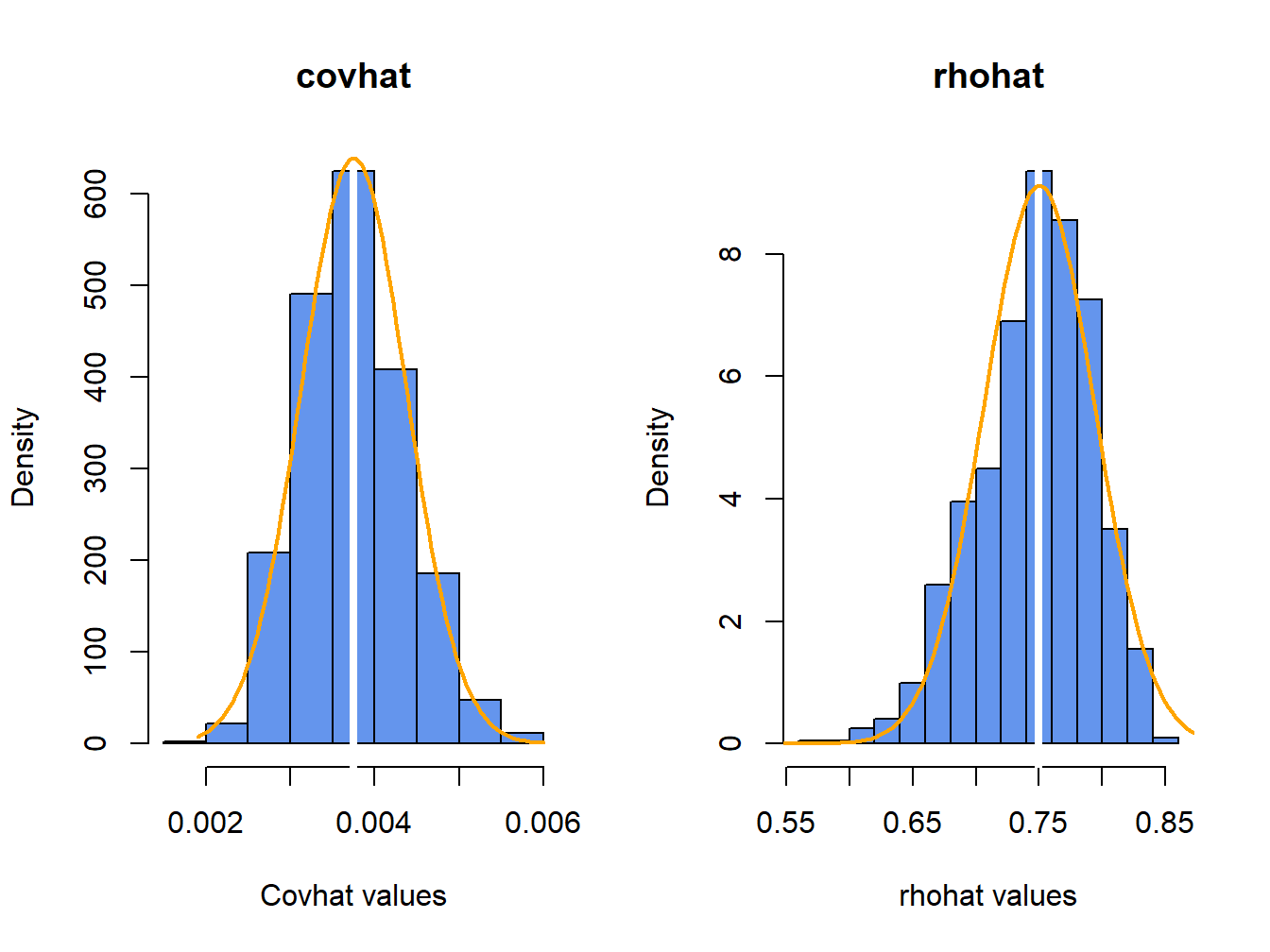
Figure 7.8: Histograms of \(\hat{\rho}_{12}\) computed from \(N=1000\) Monte Carlo samples from the bivariate GWN model (7.42) - (7.43).

The histogram for the \(\hat{\sigma}_{12}\) values is bell-shaped with and centered at the true value \(\sigma_{12}=0.00375\). The sample mean and standard deviation values of \(\hat{\sigma}_{12}\) across the 1000 simulations are, respectively, \[\begin{align*} \overline{\hat{\sigma}}_{12} & =\frac{1}{1000}\sum_{j=1}^{1000}\hat{\sigma}_{12}^{j}=0.00376,\\ \hat{\sigma}_{\hat{\sigma}_{12}} & =\sqrt{\frac{1}{999}\sum_{j=1}^{1000}(\hat{\sigma}_{12}^{j}-0.00376)^{2}}=0.000628. \end{align*}\]

Here, we see that \(\hat{\sigma_{12}}\) is essentially unbiased and the Monte Carlo standard error is almost identical to the analytic standard based the asymptotic distribution of \(\hat{\sigma}_{12}\).

The histogram for the \(\hat{\rho}_{12}\) values is bell-shaped with a mild left skewness and centered close to \(\rho_{12}=0.75\). The sample mean and standard deviation values of \(\hat{\rho}_{12}\) across the 1000 simulations are, respectively, \[\begin{align*} \overline{\hat{\rho}}_{12} & =\frac{1}{1000}\sum_{j=1}^{1000}\hat{\rho}_{12}^{j}=0.747,\\ \hat{\sigma}_{\hat{\rho}_{12}} & =\sqrt{\frac{1}{999}\sum_{j=1}^{1000}(\hat{\rho}_{12}^{j}-0.747)^{2}}=0.045. \end{align*}\]

There is very slight downward bias in \(\hat{\rho}_{12}\). The Monte Carlo standard deviation, \(\hat{\sigma}_{\hat{\rho}_{12}}\), is very close to the approximate standard error \(\mathrm{se}(\hat{\rho}_{12})=(1-0.75^{2})/\sqrt{100}=0.044\).

For each simulation \(j\), the approximate 95% confidence intervals \[\begin{align*} \hat{\sigma}_{12}^{j} & \pm2\times\widehat{\mathrm{se}}(\hat{\rho}_{12}^{j}),, \\ \hat{\rho}_{12}^{j} & \pm2\times\widehat{\mathrm{se}}(\hat{\rho}_{12}^{j}), \end{align*}\] are computed. The coverage probabilities of these interval is approximated by the fractions of intervals that contain (cover) the true values \(\sigma_{12} = 0.00375\) and \(\rho_{12}=0.75\), respectively. For the 1000 simulated samples, this fractions turns out to be 0.942 adn 0.952, respectively.

Here is the R code to support the above calculations. The Monte Carlo means, standard deviations, and analytic standard errors are:

secovhat.a = sqrt((sigmavec[1]^2*sigmavec[2]^2)*(1+rho12^2))/sqrt(n.obs)
serhohat.a = (1 - rho12^2)/sqrt(n.obs)
ans = rbind(c(cov12, mean(sim.covs),sd(sim.covs),secovhat.a),
            c(rho12, mean(sim.corrs), sd(sim.corrs), serhohat.a))
colnames(ans) = c("True Value", "MC Mean", "MC SE", "Analytic SE")
rownames(ans) = c("Covariance", "Correlation")
ans

##             True Value MC Mean    MC SE Analytic SE
## Covariance     0.00375 0.00376 0.000628    0.000625
## Correlation    0.75000 0.74685 0.045036    0.043750

The fractions of confidence intervals that cover the true parameters are:

in.interval.rho = (rho12 >= rho.lower) & (rho12 <= rho.upper)
in.interval.cov = (cov12 >= cov.lower) & (cov12 <= cov.upper)
ans = rbind(c(sum(in.interval.cov)/n.sim,0.95),
            c(sum(in.interval.rho)/n.sim,0.95))
colnames(ans) = c("MC Coverage", "True Coverage")
rownames(ans) = c("Covariance", "Correlation")
ans

##             MC Coverage True Coverage
## Covariance        0.942          0.95
## Correlation       0.952          0.95