11.2 Portfolios of Two Risky Assets

Consider the following investment problem. We can invest in two assets $A$ (Amazon stock) and $B$ (Boeing stock) over the next year, and we want to know how much to invest in each asset to make the investor most happy given the assumptions about return distributions and risk preferences from the previous sub-section. Let $R_{A}$ and $R_{B}$ denote the annual simple returns on assets $A$ and $B$ , respectively.⁶⁰ These returns are to be treated as random variables because the returns will not be realized until the end-of-the year. We assume that the returns $R_{A}$ and $R_{B}$ are jointly normally distributed, and that we have the following information about the means, variances, and covariances of the probability distribution of the two returns:

$\begin{align} \mu_{A} & =E[R_{A}],~\sigma_{A}^{2}=\mathrm{var}(R_{A}),~\mu_{B}=E[R_{B}],~\sigma_{B}^{2}=\mathrm{var}(R_{B}),\tag{11.1}\\ \sigma_{AB} & =\mathrm{cov}(R_{A},R_{B}),~\rho_{AB}=\mathrm{cor}(R_{A},R_{B})=\frac{\sigma_{AB}}{\sigma_{A}\sigma_{B}}.\tag{11.2} \end{align}$

We assume that these values are taken as given. In practice, they can be estimated from historical return data for the two stocks, or they can be subjective guesses by the investor.

The expected returns, $\mu_{A}$ and $\mu_{B}$ , are our best guesses for the annual returns on each of the assets. However, because the investment returns are random variables we must recognize that the realized returns may be different from our expectations. The variances, $\sigma_{A}^{2}$ and $\sigma_{B}^{2}$ , provide measures of the uncertainty associated with these annual returns. We can also think of the variances as measuring the risk associated with the investments. Assets with high return variability (or volatility) are often thought to be risky, and assets with low return volatility are often thought to be safe. The covariance $\sigma_{AB}$ gives us information about the direction of any linear dependence between returns. If $\sigma_{AB}>0$ then the two returns tend to move in the same direction; if $\sigma_{AB}<0$ the returns tend to move in opposite directions; if $\sigma_{AB}=0$ then the returns tend to move independently. The strength of the dependence between the returns is measured by the correlation coefficient $\rho_{AB}$ . If $\rho_{AB}$ is close to one in absolute value then returns mimic each other extremely closely, whereas if $\rho_{AB}$ is close to zero then the returns may show very little relationship.

Example 2.3 (Two risky asset portfolio information)

Table 11.1 gives annual return distribution parameters for the two hypothetical assets $A$ and $B$ that will be used in subsequent examples. Asset $A$ is the high risk asset with an annual return of $\mu_{A}=17.5\%$ and annual standard deviation of $\sigma_{A}=25.8\%$ . Asset B is a lower risk asset with annual return $\mu_{B}=5.5\%$ and annual standard deviation of $\sigma_{B}=11.5\%$ . The assets are assumed to be slightly negatively correlated with correlation coefficient $\rho_{AB}=-0.164$ .⁶¹ Given the standard deviations and the correlation, the covariance can be determined from $\sigma_{AB}=\rho_{AB}\sigma_{A}\sigma_{B}=(-0.164)(0.0258)(0.115)=-0.004875$ . In R, the example data is:⁶²

mu.A = 0.175
sig.A = 0.258
sig2.A = sig.A^2
mu.B = 0.055
sig.B = 0.115
sig2.B = sig.B^2
rho.AB = -0.164
sig.AB = rho.AB*sig.A*sig.B
data.tbl = data.frame(t(c(mu.A, mu.B, sig2.A, sig2.B, sig.A, sig.B, sig.AB, rho.AB)))
col.names = c("$\\mu_{A}$","$\\mu_{B}$","$\\sigma^{2}_{A}$","$\\sigma^{2}_{B}$",
              "$\\sigma_{A}$","$\\sigma_{B}$","$\\sigma_{AB}$","$\\rho_{AB}$")
kbl(data.tbl, col.names=col.names, caption = "Example data for two asset portfolio",
    label = "TableExampleData") %>%
   kable_styling(full_width=FALSE)

Table 11.1: Example data for two asset portfolio
$\mu_{A}$	$\mu_{B}$	$\sigma^{2}_{A}$	$\sigma^{2}_{B}$	$\sigma_{A}$	$\sigma_{B}$	$\sigma_{AB}$	$\rho_{AB}$
0.175	0.055	0.067	0.013	0.258	0.115	-0.005	-0.164

$\blacksquare$

11.2.1 The Portfolio Problem

The portfolio problem is set-up as follows. The investor has a given amount of initial wealth $W_{0}$ to be invested for one period (e.g., one month or one year). The investor can only invest in the two risky assets $A$ and $B$ and all wealth must be invested in the two assets. The investor has to decide how much wealth to put in asset $A$ and how much to put in asset $B$ . Let $x_{A}$ and $x_{B}$ denote the shares of wealth invested in assets $A$ and $B$ , respectively. The values of $x_{A}$ and $x_{B}$ can be positive or negative. Positive values denote long positions (purchases) in the assets. Negative values denote short positions (sales).⁶³ Since all wealth is put into the two investments it follows that $x_{A}+x_{B}=1$ . If asset $A$ is shorted, then it is assumed that the proceeds of the short sale are used to purchase more of asset $B$ and vice-versa.

The investment in the two assets forms a portfolio, and the shares $x_{A}$ and $x_{B}$ are referred to as portfolio shares or portfolio weights. The return on the portfolio over the next year is a random variable, and is given by:

$\begin{equation} R_{p}=x_{A}R_{A}+x_{B}R_{B},\tag{11.3} \end{equation}$

which is a linear combination or weighted average of the random variables $R_{A}$ and $R_{B}$ . Since $R_{A}$ and $R_{B}$ are assumed to be normally distributed, $R_{p}$ is also normally distributed.

Using the properties of linear combinations of random variables from Chapter 2 it follows that

$\begin{align} \mu_{p} & =E[R_{p}]=x_{A}\mu_{A}+x_{B}\mu_{B},\tag{11.4}\\ \sigma_{p}^{2} & =\mathrm{var}(R_{p})=x_{A}^{2}\sigma_{A}^{2}+x_{B}^{2}\sigma_{B}^{2}+2x_{A}x_{B}\sigma_{AB},\tag{11.5}\\ \sigma_{p} & =\mathrm{SD}(R_{p})=\sqrt{x_{A}^{2}\sigma_{A}^{2}+x_{B}^{2}\sigma_{B}^{2}+2x_{A}x_{B}\sigma_{AB}}.\tag{11.6} \end{align}$

Hence, the portfolio return has the following normal distribution: $R_{p}\sim N(\mu_{p},\sigma_{p}^{2}).$

Given the portfolio return distribution, end-of-period wealth is

$\begin{equation*} W_{1} = W_{0}\times (1 + R_{p}) = W_{0}+ W_{0}\times R_{p}, \end{equation*}$

which is a linear function of the random portfolio return $R_{p}$ . It follows that

$\begin{align*} E[W_{1}] &= W_{0} + W_{0}\times E[R_{p}] = W_{0}(1 + \mu_{p}), \\ \mathrm{var}(W_{1}) &= W_{0}^{2}\times \mathrm{var}(R_{p}) = W_{0}^{2}\times \sigma_{p}^2, \end{align*}$

so that the distribution of $W_{1}$ is normal:

$\begin{equation*} W_{1} \sim N(W_{0}(1 + \mu_{p}), W_{0}^{2}\times \sigma_{p}^2). \end{equation*}$

The investor cares most about the distribution of end-of-period wealth $W_{1}$ , which depends on the values of $W_{0}$ , $\mu_{p}$ , and $\sigma_{p}^2$ . Since $\mu_{p}$ and $\sigma_{p}^2$ are functions of $x_{A}$ and $x_{B}$ , the portfolio problem is to find the values of $x_{A}$ and $x_{B}$ that makes the investor most happy with respect to the probability distribution of end-of-period wealth.⁶⁴

The results (11.4) and (11.5) are so important to portfolio theory that it is worthwhile to review the derivations.⁶⁵ For the first result (11.4), we have: $E[R_{p}]=E[x_{A}R_{A}+x_{B}R_{B}]=x_{A}E[R_{A}]+x_{B}E[R_{B}]=x_{A}\mu_{A}+x_{B}\mu_{B},$ by the linearity of the expectation operator. For the second result (11.5), we have: $\begin{align*} \mathrm{var}(R_{p}) & =E[(R_{p}-\mu_{p})^{2}]=E[(x_{A}(R_{A}-\mu_{A})+x_{B}(R_{B}-\mu_{B}))^{2}]\\ & =E[x_{A}^{2}(R_{A}-\mu_{A})^{2}+x_{B}^{2}(R_{B}-\mu_{B})^{2}+2x_{A}x_{B}(R_{A}-\mu_{A})(R_{B}-\mu_{B})]\\ & =x_{A}^{2}E[(R_{A}-\mu_{A})^{2}]+x_{B}^{2}E[(R_{B}-\mu_{B})^{2}]+2x_{A}x_{B}E[(R_{A}-\mu_{A})(R_{B}-\mu_{B})]\\ & =x_{A}^{2}\sigma_{A}^{2}+x_{B}^{2}\sigma_{B}^{2}+2x_{A}x_{B}\sigma_{AB}. \end{align*}$

The third line uses linearity of the expectations operator, and the fourth line uses the definition of variance and covariance.

Notice that the variance of the portfolio is a weighted average of the variances of the individual assets plus two times the product of the portfolio weights times the covariance between the assets. If the portfolio weights are both positive then a positive covariance will tend to increase the portfolio variance, because both returns tend to move in the same direction, and a negative covariance will tend to reduce the portfolio variance as returns tend to move in opposite directions. Thus finding assets with negatively correlated returns can be very beneficial when forming portfolios because risk, as measured by portfolio standard deviation, can be reduced. What is perhaps surprising is that forming portfolios with positively correlated assets can also reduce risk as long as the correlation is not too large. We illustrate these results with the following examples.

Example 4.2 (Two asset portfolios)

Consider creating some portfolios using the asset information in Table 11.1. The first portfolio is an equally weighted portfolio with $x_{A}=x_{B}=0.5$ . Using (11.4)-(11.6), we have: $\begin{align*} \mu_{p_{1}} & =(0.5)\cdot(0.175)+(0.5)\cdot(0.055)=0.115\\ \sigma_{p_{1}}^{2} & =(0.5)^{2}\cdot(0.067)+(0.5)^{2}\cdot(0.013)\\ & +2\cdot(0.5)(0.5)(-0.004866)\\ & =0.01751\\ \sigma_{p_{1}} & =\sqrt{0.01751}=0.1323 \end{align*}$ This portfolio has expected return half-way between the expected returns on assets $A$ and $B$ , but the portfolio standard deviation is less than half-way between the asset standard deviations. This reflects risk reduction via diversification. Here, diversification means investing wealth in two assets instead of investing wealth in a single asset. In R, the portfolio parameters are computed using:

x.A = 0.5
x.B = 0.5
mu.p1 = x.A*mu.A + x.B*mu.B
sig2.p1 = x.A^2 * sig2.A + x.B^2 * sig2.B + 2*x.A*x.B*sig.AB
sig.p1 = sqrt(sig2.p1)
data.tbl = t(c(mu.p1, sig.p1, 0.5*sig.A+0.5*sig.B))
col.names = c("$\\mu_{p_{1}}$", "$\\sigma_{p_{1}}$", "$0.5\\sigma_{A}+0.5\\sigma_{B}$")
kbl(data.tbl, col.names=col.names) %>%
   kable_styling(full_width=FALSE)

$\mu_{p_{1}}$	$\sigma_{p_{1}}$	$0.5\sigma_{A}+0.5\sigma_{B}$
0.115	0.132	0.186

Next, consider a long-short portfolio with $x_{A}=1.5$ and $x_{B}=-0.5$ . In this portfolio, asset $B$ is sold short and the proceeds of the short sale are used to leverage the investment in asset $A$ .⁶⁶ The portfolio characteristics are: $\begin{align*} \mu_{p_{2}} & =(1.5)\cdot(0.175)+(-0.5)\cdot(0.055)=0.235\\ \sigma_{p_{2}}^{2} & =(1.5)^{2}\cdot(0.067)+(-0.5)^{2}\cdot(0.013)\\ & +2\cdot(1.5)(-0.5)(-0.004866)\\ & =0.1604\\ \sigma_{p_{2}} & =\sqrt{0.1604}=0.4005 \end{align*}$ This portfolio has both a higher expected return and standard deviation than asset $A$ . The high standard deviation is due to the short sale, which is a type of leverage, and the negative correlation between assets $A$ and $B$ . In R, the portfolio parameters are computed using:

x.A = 1.5
x.B = -0.5
mu.p2 = x.A*mu.A + x.B*mu.B
sig2.p2 = x.A^2 * sig2.A + x.B^2 * sig2.B + 2*x.A*x.B*sig.AB
sig.p2 = sqrt(sig2.p2)
data.tbl = t(c(mu.p2, sig.p2, 1.5*sig.A-0.5*sig.B))
col.names = c("$\\mu_{p_{2}}$", "$\\sigma_{p_{2}}$", "$1.5\\sigma_{A}-0.5\\sigma_{B}$")
kbl(data.tbl, col.names=col.names) %>%
   kable_styling(full_width=FALSE)

$\mu_{p_{2}}$	$\sigma_{p_{2}}$	$1.5\sigma_{A}-0.5\sigma_{B}$
0.235	0.4	0.33

$\blacksquare$

In the above example, the equally weighted portfolio has expected return half way between the expected returns on assets A and B, but has standard deviation (volatility) that is less than half way between the standard deviations of the two assets. For long-only portfolios, we can show that this is a general result as long as the correlation between the two assets is not perfectly positive.

Proposition 11.1 Consider a portfolio of the two assets A and B with portfolios weights $x_{A}\geq0$ and $x_{B}\geq0$ such that $x_{A}+x_{B}=1.$ Then if $\rho_{AB}\neq1$

$\sigma_{p}=(x_{A}^{2}\sigma_{A}^{2}+x_{B}^{2}\sigma_{B}^{2}+2x_{A}x_{B}\sigma_{AB})^{1/2}<x_{A}\sigma_{A}+x_{B}\sigma_{B}.$

If $\rho_{AB}=1$ then

$\sigma_{p}=x_{A}\sigma_{A}+x_{B}\sigma_{B}.$

The proof is straightforward. Use $\sigma_{AB}=\rho_{AB}\sigma_{A}\sigma_{B}$ and write

$\sigma_{p}^{2}=x_{A}^{2}\sigma_{A}^{2}+x_{B}^{2}\sigma_{B}^{2}+2x_{A}x_{B}\sigma_{AB}=x_{A}^{2}\sigma_{A}^{2}+x_{B}^{2}\sigma_{B}^{2}+2x_{A}x_{B}\rho_{AB}\sigma_{A}\sigma_{B}.$

Now add and subtract $2x_{A}x_{B}\sigma_{A}\sigma_{B}$ from the right-hand side to give $\begin{eqnarray*} \sigma_{p}^{2} & = & (x_{A}^{2}\sigma_{A}^{2}+x_{B}^{2}\sigma_{B}^{2}+2x_{A}x_{B}\sigma_{A}\sigma_{B})-2x_{A}x_{B}\sigma_{A}\sigma_{B}+2x_{A}x_{B}\rho_{AB}\sigma_{A}\sigma_{B}\\ & = & \left(x_{A}\sigma_{A}+x_{B}\sigma_{B}\right)^{2}-2x_{A}x_{B}\sigma_{A}\sigma_{B}(1-\rho_{AB}). \end{eqnarray*}$ If $\rho_{AB}\neq1$ then $2x_{A}x_{B}\sigma_{A}\sigma_{B}(1-\rho_{AB})>0$ and so $\sigma_{p}^{2}<\left(x_{A}\sigma_{A}+x_{B}\sigma_{B}\right)^{2}\Rightarrow\sigma_{p}<x_{A}\sigma_{A}+x_{B}\sigma_{B}.$

If $\rho_{AB}=1$ then $2x_{A}x_{B}\sigma_{A}\sigma_{B}(1-\rho_{AB})=0$ and $\sigma_{p}^{2}=\left(x_{A}\sigma_{A}+x_{B}\sigma_{B}\right)\Rightarrow\sigma_{p}=x_{A}\sigma_{A}+x_{B}\sigma_{B}$ This result shows that the volatility of a long-only two asset portfolio is a weighted average of individual asset volatility only when the two assets have perfectly positively correlated returns. Hence, in this case there is no risk reduction benefit from forming a portfolio. However, if assets are not perfectly correlated then there can be a risk reduction benefit from forming a portfolio. How big the risk reduction benefit is depends on the magnitude of the asset return correlation $\rho_{AB}$ . In general, the closer $\rho_{AB}$ is to -1 the larger is the risk reduction benefit.

Figure 11.1 shows the risk-return characteristics of assets A and B as well as the equally weighted and long-short portfolios (labeled P1 and P2, respectively). The dotted line connecting the points A and B represents linear risk-return trade-offs of portfolios of assets A and B, respectively, that occurs if $\rho_{AB}=1$ . The point P1, which represents the equally weighted long-only portfolio, has expected return half-way between the expected returns on assets A and B but has standard deviation less than half-way between the standard deviations of assets A and B. As a result, P1 lies to the left of the dotted line indicating a risk reduction benefit to the portfolio. In contrast, the point P2, which represents the long-short portfolio, lies to the right of the dotted line indicating a risk inflation cost of the portfolio due to leverage.

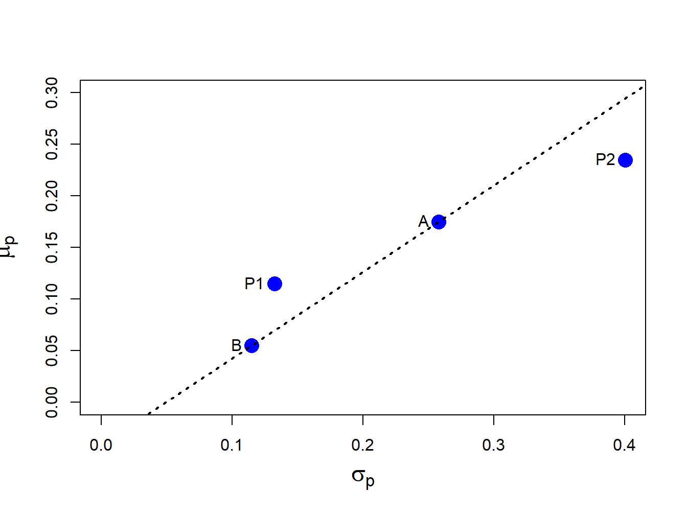
Figure 11.1: Risk-return characteristics of assets A and B, the equally weighted portfolio P1 and the long-short portfolio P2.

11.2.2 Portfolio Value-at-Risk

Consider an initial investment of $\$W_{0}$ in the portfolio of assets $A$ and $B$ with return given by (11.3), expected return given by (11.4)) and variance given by (11.5). Then $R_{p}\sim N(\mu_{p},\sigma_{p}^{2})$ . For $\alpha\in(0,1)$ , the $\alpha\times100\%$ portfolio value-at-risk is given by:

$\begin{equation} \mathrm{VaR}_{p,\alpha}= -q_{\alpha}^{R_{p}}W_{0},\tag{11.7} \end{equation}$

where $q_{\alpha}^{R_{p}}$ is the $\alpha$ -quantile of the distribution of $R_{p}$ and is given by

$\begin{equation} q_{\alpha}^{R_{p}}=\mu_{p}+\sigma_{p}q_{\alpha}^{z},\tag{11.8} \end{equation}$

where $q_{\alpha}^{z}$ is the $\alpha$ -quantile of the standard normal distribution.⁶⁷

What is the relationship between portfolio VaR and the individual asset VaRs? Is portfolio VaR a weighted average of the individual asset VaRs? In general, portfolio VaR is not a weighted average of the asset VaRs. To see this consider the portfolio weighted average of the individual asset return quantiles:

$\begin{align} x_{A}q_{\alpha}^{R_{A}}+x_{B}q_{\alpha}^{R_{B}} & =x_{A}(\mu_{A}+\sigma_{A}q_{\alpha}^{z})+x_{B}(\mu_{B}+\sigma_{B}q_{\alpha}^{z})\nonumber \\ & =x_{A}\mu_{A}+x_{B}\mu_{B}+(x_{A}\sigma_{A}+x_{B}\sigma_{B})q_{\alpha}^{z}\nonumber \\ & =\mu_{p}+(x_{A}\sigma_{A}+x_{B}\sigma_{B})q_{\alpha}^{z}.\tag{11.9} \end{align}$

The weighted asset quantile (11.9) is not equal to the portfolio quantile (11.8) unless $\rho_{AB}=1$ . Hence, weighted asset VaR is in general not equal to portfolio VaR because the quantile (11.9) assumes a perfectly positive correlation between $R_{A}$ and $R_{B}$ .

Example 2.5 (Portfolio VaR)

Consider an initial investment of $W_{0}=\$100,000$ . Assuming that returns are simple, the 5% VaRs on assets $A$ and $B$ are:

$\begin{align*} \mathrm{VaR}_{A,0.05} & = -q_{0.05}^{R_{A}}W_{0}= -\left(\mu_{A}+\sigma_{A}q_{.05}^{z}\right)W_{0}\\ & = -(0.175+0.258(-1.645))\cdot100,000= 24,937,\\ \mathrm{VaR}_{B,0.05} & = -q_{0.05}^{R_{B}}W_{0}= -\left(\mu_{B}+\sigma_{B}q_{.05}^{z}\right)W_{0}\\ & = -(0.055+0.115(-1.645))\cdot100,000= 13,416. \end{align*}$

The 5% VaR on the equal weighted portfolio with $x_{A}=x_{B}=0.5$ is:

$\begin{align*} \mathrm{VaR}_{p,0.05} & = -q_{0.05}^{R_{p}}W_{0}= -\left(\mu_{p}+\sigma_{p}q_{.05}^{z}\right)W_{0}\\ & = -(0.115+0.1323(-1.645))\cdot100,000= 10,268, \end{align*}$

and the weighted average of the individual asset VaRs is, $x_{A}\mathrm{VaR}_{A,0.05}+x_{B}\mathrm{VaR}_{B,0.05}=0.5(24,937)+0.5(13,416)=19,177.$ The 5% VaR on the long-short portfolio with $x_{A}=1.5$ and $x_{B}=-0.5$ is: $\mathrm{VaR}_{p,0.05}= -q_{0.05}^{R_{p}}W_{0}= -(0.235+0.4005(-1.645))\cdot100,000=42,371,$ and the weighted average of the individual asset VaRs is, $x_{A}\mathrm{VaR}_{A,0.05}+x_{B}\mathrm{VaR}_{B,0.05}=1.5(24,937)-0.5(13,416)=30,698.$ Notice that VaR $_{p,0.05}\neq x_{A}\mathrm{VaR}_{A,0.05}+x_{B}\mathrm{VaR}_{B,0.05}$ because $\rho_{AB}\neq1$ .

Using R, these computations are:

w0 = 100000
VaR.A = -(mu.A + sig.A*qnorm(0.05))*w0
VaR.B = -(mu.B + sig.B*qnorm(0.05))*w0
VaR.p1 = -(mu.p1 + sig.p1*qnorm(0.05))*w0
VaR.p2 = -(mu.p2 + sig.p2*qnorm(0.05))*w0
data.tbl = t(c(VaR.A,VaR.B,VaR.p1,VaR.p2))
col.names = c("$VaR_{A,0.05}$", "$VaR_{B,0.05}$", "$VaR_{p_{1},0.05}$",
              "$VaR_{p_{2},0.05}$")
kbl(data.tbl, col.names=col.names) %>%
   kable_styling(full_width=FALSE)

$VaR_{A,0.05}$	$VaR_{B,0.05}$	$VaR_{p_{1},0.05}$	$VaR_{p_{2},0.05}$
24937	13416	10268	42371

data.tbl = t(c(0.5*VaR.A+0.5*VaR.B,1.5*VaR.A-0.5*VaR.B))
col.names = c("$0.5VaR_{A,0.05}+0.5VaR_{B,0.05}$",
              "$1.5VaR_{A,0.05}-0.5VaR_{B,0.05}$")
kbl(data.tbl, col.names=col.names) %>%
   kable_styling(full_width=FALSE)

$0.5VaR_{A,0.05}+0.5VaR_{B,0.05}$	$1.5VaR_{A,0.05}-0.5VaR_{B,0.05}$
19177	30698

$\blacksquare$

Example 2.7 (Create R function to compute normal VaR)

The previous example used repetitive R calculations to compute the 5% VaR for a variety of investments. An alternative approach is to create an R function to compute the VaR given $\mu$ , $\sigma$ , $\alpha$ (VaR probability) and $W_{0}$ , and then apply the function using the inputs of the different assets. A simple function to compute VaR based on normally distributed asset returns is:

normalVaR = function(mu, sigma, w0, alpha = 0.05, invert=TRUE) {
## compute normal VaR for collection of assets given mean and sd vector
## inputs:
## mu         n x 1 vector of expected returns
## sigma      n x 1 vector of standard deviations
## w0         scalar initial investment in $
## alpha      scalar tail probability
## invert     logical. If TRUE report VaR as positive number
## output:
## VaR        n x 1 vector of left tail return quantiles
  if ( length(mu) != length(sigma) )
    stop("mu and sigma must have same number of elements")
  if ( alpha < 0 || alpha > 1)
    stop("alpha must be between 0 and 1")
  VaR = w0*(mu + sigma*qnorm(alpha))
  if (invert) {
    VaR = -VaR
  }
  return(VaR)
}

You create an R function using function(). Every R function has a set of arguments or inputs. Here, the arguments are the $n \times 1$ vectors mu and sigma, the scalars w0 and alpha, and the logical value invert. Default values for alpha and invert are specified in the definition of the function. The body of the function is defined within the braces {}, and the return value of the function is specified using return(). Here, we first check that the inputs mu and sigma are of the same length, and that the tail probability $\alpha$ is between 0 and 1. Then, we compute normal VaR using (11.7). If invert=TRUE we multiply the result by $-1$ . Finally, we return the vector of VaR values. After running the code that defines the function normalVaR(), it will be available in the R session for use like any other R function.

Using the normalVaR() function, the 5% VaR values of asset $A$ , $B$ and equally weighted portfolio are:

normalVaR(mu=c(mu.A, mu.B, mu.p1),
          sigma=c(sig.A, sig.B, sig.p1),
          w0=100000, alpha=0.05)

## [1] 24937 13416 10268

$\blacksquare$

11.2.3 The set of feasible portfolios

The collection of all feasible portfolios, or the investment possibilities set, in the case of two assets is simply all possible portfolios that can be formed by varying the portfolio weights $x_{A}$ and $x_{B}$ such that the weights sum to one ( $x_{A}+x_{B}=1)$ . We summarize the expected return-risk (mean-volatility) properties of the feasible portfolios in a plot with portfolio expected return, $\mu_{p}$ , on the vertical axis and portfolio standard deviation, $\sigma_{p}$ , on the horizontal axis. The portfolio standard deviation is used instead of variance because standard deviation is measured in the same units as the expected value (recall, variance is the average squared deviation from the mean).

Example 2.9 (Investment possibilities set for example data)

The investment possibilities set for the data in Table 11.1 is illustrated in Figure 11.2. Here the portfolio weight on asset A, $x_{A}$ , is varied from -0.4 to 1.4 in increments of 0.1 and, since $x_{B}=1-x_{A}$ , the weight on asset B then varies from 1.4 to -0.4. This gives us 18 portfolios with weights $(x_{A},x_{B})=(-0.4,1.4),(-0.3,1.3),...,(1.3,-0.3),(1.4,-0.4)$ . For each of these portfolios we use the formulas (11.4) and (11.6) to compute $\mu_{p}$ and $\sigma_{p}$ . In R, the calculations are:

x.A = seq(from=-0.4, to=1.4, by=0.1)
x.B = 1 - x.A
mu.p = x.A*mu.A + x.B*mu.B
sig2.p = x.A^2 * sig2.A + x.B^2 * sig2.B + 2*x.A*x.B*sig.AB
sig.p = sqrt(sig2.p)
port.names = paste("portfolio", 1:length(x.A), sep=" ")
data.tbl = as.data.frame(cbind(x.A, x.B, mu.p, sig.p))
rownames(data.tbl) = port.names
col.names = c("$x_{A}$","$x_{B}$", "$\\mu_{p}$", "$\\sigma_{p}$" )
kbl(data.tbl, col.names=col.names) %>%
   kable_styling(full_width=FALSE)

	$x_{A}$	$x_{B}$	$\mu_{p}$	$\sigma_{p}$
portfolio 1	-0.4	1.4	0.007	0.205
portfolio 2	-0.3	1.3	0.019	0.179
portfolio 3	-0.2	1.2	0.031	0.155
portfolio 4	-0.1	1.1	0.043	0.133
portfolio 5	0.0	1.0	0.055	0.115
portfolio 6	0.1	0.9	0.067	0.102
portfolio 7	0.2	0.8	0.079	0.098
portfolio 8	0.3	0.7	0.091	0.102
portfolio 9	0.4	0.6	0.103	0.114
portfolio 10	0.5	0.5	0.115	0.132
portfolio 11	0.6	0.4	0.127	0.154
portfolio 12	0.7	0.3	0.139	0.178
portfolio 13	0.8	0.2	0.151	0.204
portfolio 14	0.9	0.1	0.163	0.231
portfolio 15	1.0	0.0	0.175	0.258
portfolio 16	1.1	-0.1	0.187	0.286
portfolio 17	1.2	-0.2	0.199	0.314
portfolio 18	1.3	-0.3	0.211	0.343
portfolio 19	1.4	-0.4	0.223	0.372

Portfolios 1-4 and 16-19 are the long-short portfolios and portfolios 5-15 are the long-only portfolios. In R, the risk-return properties of this set of feasible portfolios can be visualized using:

cex.val = 1.5
plot(sig.p, mu.p, type="b", pch=16, cex=cex.val,
     ylim=c(0, max(mu.p)), xlim=c(0, max(sig.p)), 
     xlab=expression(sigma[p]), ylab=expression(mu[p]),
     cex.lab=1.5, col=c(rep("blue", 4), rep("black", 2),
                        "green", rep("black", 8), rep("blue", 4)))
text(x=sig.A, y=mu.A, labels="Asset A", pos=4)
text(x=sig.B, y=mu.B, labels="Asset B", pos=4)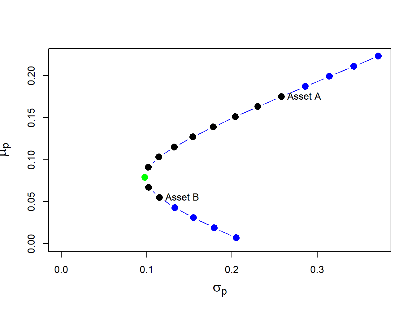

Figure 11.2: Portfolio frontier of example data.

$\blacksquare$

Notice that the plot in ( $\mu_{p},\sigma_{p})$ -space looks like a parabola turned on its side (in fact, it is one side of a hyperbola). The plot is often referred to as the Markowitz bullet as it resembles the shape of a bullet speeding toward the y-axis. The black dots plus the green dot represent the long-only portfolios, and the blue dots represent long-short portfolios. The black dot labeled “Asset A” is the portfolio $(x_{A}=1, x_{B}=0)$ , and the black dot labeled “Asset B” is the portfolio $(x_{A}=0, x_{B}=1)$ .

The bullet shape of the feasible set shows that portfolio risk can be reduced through diversification. Risk reduction through diversification can be understood as follows. Suppose an investor is initially invested 100% in asset B (i.e., portfolio 5). Diversification involves rebalancing the portfolio to include asset A. For example, portfolio 6 is $(x_{A}=0.1, x_{B}=0.9)$ . This portfolio has both a higher expected return and a lower standard deviation than portfolio 5. This is the benefit from diversification. Portfolio expected return increases and risk decreases until portfolio 7 is reached, which is at the tip of the Markowitz bullet (green dot). This portfolio has the property that it has the smallest variance/volatility among all feasible portfolios. Accordingly, this portfolio is called the global minimum variance portfolio. Continuing from portfolio 8 through portfolio 19, we see that both expected return and risk increase.

11.2.4 Computing the global minimum variance portfolio

The global minimum variance portfolio plays a key role in mean-variance portfolio theory and it is important to know how to determine its weights. Here, we show that it is a simple exercise in calculus to find the global minimum variance portfolio weights. We solve the constrained optimization problem⁶⁸:

$\begin{align*} \underset{x_{A},x_{B}}{\min}\sigma_{p}^{2} & =x_{A}^{2}\sigma_{A}^{2}+x_{B}^{2}\sigma_{B}^{2}+2x_{A}x_{B}\sigma_{AB}\\ ~s.t.~x_{A}+x_{B} & =1. \end{align*}$

This constrained optimization problem can be solved using two methods. The first method, called the method of substitution, uses the constraint to substitute out one of the variables to transform the constrained optimization problem in two variables into an unconstrained optimization problem in one variable. The second method, called the method of Lagrange multipliers, introduces an auxiliary variable called the Lagrange multiplier and transforms the constrained optimization problem in two variables into an unconstrained optimization problem in three variables.

The substitution method is straightforward. Substituting $x_{B}=1-x_{A}$ into the formula for $\sigma_{p}^{2}$ reduces the problem to: $\min_{x_{A}}\sigma_{p}^{2}=x_{A}^{2}\sigma_{A}^{2}+(1-x_{A})^{2}\sigma_{B}^{2}+2x_{A}(1-x_{A})\sigma_{AB}.$ The first order conditions for a minimum, via the chain rule, are: $0=\frac{d\sigma_{p}^{2}}{dx_{A}}=2x_{A}^{\min}\sigma_{A}^{2}-2(1-x_{A}^{\min})\sigma_{B}^{2}+2\sigma_{AB}(1-2x_{A}^{\min}),$ and straightforward calculations yield,

$\begin{equation} x_{A}^{\min}=\frac{\sigma_{B}^{2}-\sigma_{AB}}{\sigma_{A}^{2}+\sigma_{B}^{2}-2\sigma_{AB}},~x_{B}^{\min}=1-x_{A}^{\min}.\tag{11.10} \end{equation}$

The method of Lagrange multipliers involves two steps. In the first step, the constraint $x_{A}+x_{B}=1$ is put into homogenous form $x_{A}+x_{B}-1=0$ . In the second step, the Lagrangian function is formed by adding to $\sigma_{p}^{2}$ the homogenous constraint multiplied by an auxiliary variable $\lambda$ (the Lagrange multiplier) giving: $L(x_{A},x_{B},\lambda)=x_{A}^{2}\sigma_{A}^{2}+x_{B}^{2}\sigma_{B}^{2}+2x_{A}x_{B}\sigma_{AB}+\lambda(x_{A}+x_{B}-1).$ This function is then minimized with respect to $x_{A},$ $x_{B}$ , and $\lambda$ . The first order conditions are:

$\begin{align*} 0 & =\frac{\partial L(x_{A},x_{B},\lambda)}{\partial x_{A}}=2x_{A}\sigma_{A}^{2}+2x_{B}\sigma_{AB}+\lambda,\\ 0 & =\frac{\partial L(x_{A},x_{B},\lambda)}{\partial x_{B}}=2x_{B}\sigma_{B}^{2}+2x_{A}\sigma_{AB}+\lambda,\\ 0 & =\frac{\partial L(x_{A},x_{B},\lambda)}{\partial\lambda}=x_{A}+x_{B}-1. \end{align*}$

The first two equations can be rearranged to give: $x_{B}=x_{A}\left(\frac{\sigma_{A}^{2}-\sigma_{AB}}{\sigma_{B}^{2}-\sigma_{AB}}\right).$ Substituting this value for $x_{B}$ into the third equation and rearranging gives the solution (11.10).

Example 2.11 (Global minimum variance portfolio for example data)

Using the data in Table 11.1 and (11.10) we have: $x_{A}^{\min}=\frac{0.01323-(-0.004866)}{0.06656+0.01323-2(-0.004866)}=0.2021,~x_{B}^{\min}=0.7979.$ Hence, the global minimum variance portfolio is essentially portfolio 7 in Figure 11.2 and indeed lies at the tip of the Markowitz bullet.

The expected return, variance and standard deviation of this portfolio are:

$\begin{align*} \mu_{p} & =(0.2021)\cdot(0.175)+(0.7979)\cdot(0.055)=0.07925\\ \sigma_{p}^{2} & =(0.2021)^{2}\cdot(0.067)+(0.7979)^{2}\cdot(0.013)\\ & +2\cdot(0.2021)(0.7979)(-0.004875)\\ & =0.00975\\ \sigma_{p} & =\sqrt{0.00975}=0.09782. \end{align*}$

In R, the calculations to compute the global minimum variance portfolio weights and its expected return and volatility are:

xA.min = (sig2.B - sig.AB)/(sig2.A + sig2.B - 2*sig.AB)
xB.min = 1 - xA.min
mu.p.min = xA.min*mu.A + xB.min*mu.B
sig2.p.min = xA.min^2 * sig2.A + xB.min^2 * sig2.B + 2*xA.min*xB.min*sig.AB
sig.p.min = sqrt(sig2.p.min)
data.tbl = as.data.frame(t(c(xA.min, xB.min, mu.p.min, sig.p.min)))
col.names = c("$x_{A}^{\\min}$","$x_{B}^{\\min}$", "$\\mu_{p}^{\\min}$", 
              "$\\sigma_{p}^{\\min}$" )
kbl(data.tbl, col.names=col.names) %>%
   kable_styling(full_width=FALSE)

$x_{A}^{\min}$	$x_{B}^{\min}$	$\mu_{p}^{\min}$	$\sigma_{p}^{\min}$
0.202	0.798	0.079	0.098

$\blacksquare$

11.2.5 Correlation and the shape of the portfolio frontier

The shape of the investment possibilities set is very sensitive to the correlation between assets $A$ and $B$ given the other parameters. We illustrate this sensitivity by computing portfolio frontiers for the example data for $\rho_{AB} = -0.9, -0.5, 0, 0.5, 0.9$ . Figure 11.3 shows these portfolio frontiers.

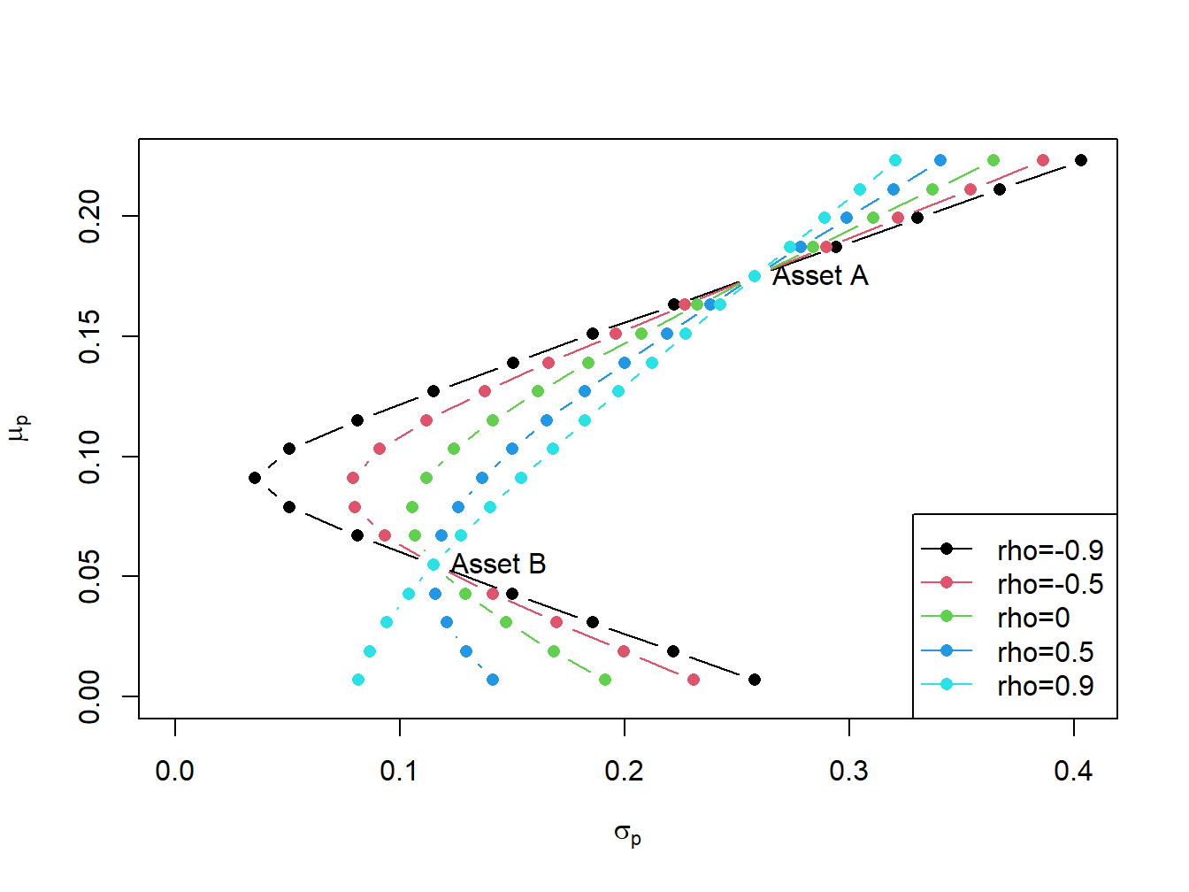
Figure 11.3: Portfolio frontier as a function of correlation.

The curvature of the portfolio frontier is determined by the value of $\rho_{AB}$ . The closer $\rho_{AB}$ is to -1 the more curved is the frontier toward the y-axis and the higher is the possible diversification benefit. What is perhaps surprising from Figure 11.3 is that there is noticeable curvature even for positive values of $\rho_{AB}$ .

$Portfolios with $\rho_{AB}=1$ and $\rho_{AB}=-1$.$

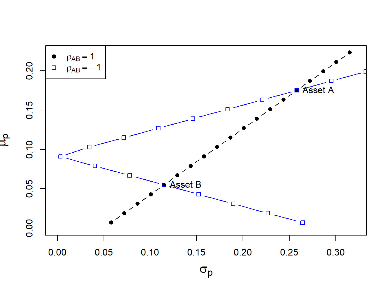
Figure 11.4: Portfolios with $\rho_{AB}=1$ and $\rho_{AB}=-1$ .

If $\rho_{AB}$ is close to 1 then the portfolio frontier approaches a straight line connecting the portfolio with all wealth invested in asset $B$ , $(x_{A},x_{B})=(0,1)$ , to the portfolio with all wealth invested in asset $A$ , $(x_{A},x_{B})=(1,0)$ . If $\rho_{AB}=-1$ then the set actually touches the $\mu_{p}$ axis. What this means is that if assets $A$ and $B$ are perfectly negatively correlated then there exists a portfolio of $A$ and $B$ that has positive expected return and zero variance! These cases are illustrated in Figure 11.4.

To find the portfolio with $\sigma_{p}^{2}=0$ when $\rho_{AB}=-1$ we use (11.10) and the fact that $\sigma_{AB}=\rho_{AB}\sigma_{A}\sigma_{B}$ to give: $x_{A}^{\min}=\frac{\sigma_{B}}{\sigma_{A}+\sigma_{B}},~x_{B}^{\min}=1-x_{A}.$

If the stocks pay a dividend then returns are computed as total returns.↩︎
The small negative correlation between the two stock returns is a bit unusual, as most stock returns are positively correlated. The negative correlation is assumed so that certain figures produced later look nice and are easy to read. ↩︎
We use the kableExtra function kbl() to print out nice formatted tables from a data.frame of information.↩︎
To short an asset one borrows the asset, usually from a broker, and then sells it. The proceeds from the short sale are usually kept on account with a broker and there may be restrictions on the use of these funds for the purchase of other assets. The short position is closed out when the asset is repurchased and then returned to original owner. If the asset drops in value then a gain is made on the short sale and if the asset increases in value a loss is made. See Chapter 13 for more details on short selling assets↩︎
In formal terms, the portfolio problem is to find the values of $x_{A}$ and $x_{B}$ that maximizes the investor’s expected utility over end-of-period wealth↩︎
See chapter 2 section 2.1.↩︎
Leverage refers to an investment that is financed through borrowing. Here, the short sale of asset B produces borrowed funds used to purchase more of asset A. This increases the risk (portfolio standard deviation) of the investment.↩︎
If $R_{p}$ is a continuously compounded return then the implied simple return quantile is $q_{\alpha}^{R_{p}}=\exp(\mu_{p}+\sigma_{p}q_{\alpha}^{z})-1$ .↩︎
A review of optimization and constrained optimization is given in the appendix to this chapter.↩︎