4.3 Time Series Models
Time series models are probability models that are used to describe the behavior of a stochastic process. In many cases of interest, it is assumed that the stochastic process to be modeled is covariance stationary and ergodic. Then, the main feature of the process to be modeled is the time dependence between the random variables. In this section, we illustrate some simple models for covariance stationary and ergodic time series that exhibit particular types of linear time dependence captured by autocorrelations. The univariate models, made popular originally by (Box and Jenkins 1976), are called autoregressive moving average (ARMA) models. The multivariate model, made popular by (Sims 1980), is called the vector autoregressive (VAR) model. These models are used extensively in economics and finance for modeling univariate and multivariate time series.
4.3.1 Moving average models
Moving average models are simple covariance stationary and ergodic time series models built from linear functions of GWN that can capture time dependence between random variables that lasts only for a finite number of lags.
4.3.1.1 MA(1) Model
Suppose you want to create a covariance stationary and ergodic stochastic process \(\{Y_{t}\}\) in which \(Y_{t}\) and \(Y_{t-1}\) are correlated but \(Y_{t}\) and \(Y_{t-j}\) are not correlated for \(j>1.\) That is, the time dependence in the process only lasts for one period. Such a process can be created using the first order moving average (MA(1)) model: \[\begin{align} Y_{t} & =\mu+\varepsilon_{t}+\theta\varepsilon_{t-1},~-1<\theta<1,\tag{4.2}\\ & \varepsilon_{t}\sim\mathrm{GWN}(0,\sigma_{\varepsilon}^{2}).\nonumber \end{align}\] The MA(1) model is a simple linear function of the GWN random variables \(\varepsilon_{t}\) and \(\varepsilon_{t-1}.\) This linear structure allows for easy analysis of the model. The moving average parameter \(\theta\) determines the sign and magnitude of the correlation between \(Y_{t}\) and \(Y_{t-1}\). Clearly, if \(\theta=0\) then \(Y_{t}=\mu+\varepsilon_{t}\) so that \(\{Y_{t}\}\) is GWN with non-zero mean \(\mu\) and exhibits no time dependence. As will be shown below, the MA(1) model produces a covariance stationary and ergodic process for any (finite) value of \(\theta\). The restriction \(-1<\theta<1\) is called the invertibility restriction and will be explained below.
To verify that (4.2) process is a covariance stationary process we must show that the mean, variance and autocovariances are time invariant. For the mean, we have: \[ E[Y_{t}]=\mu+E[\varepsilon_{t}]+\theta E[\varepsilon_{t-1}]=\mu, \] because \(E[\varepsilon_{t}]=E[\varepsilon_{t-1}]=0\).
For the variance, we have \[\begin{align*} \mathrm{var}(Y_{t}) & =\sigma^{2}=E[(Y_{t}-\mu)^{2}]=E[(\varepsilon_{t}+\theta\varepsilon_{t-1})^{2}]\\ & =E[\varepsilon_{t}^{2}]+2\theta E[\varepsilon_{t}\varepsilon_{t-1}]+\theta^{2}E[\varepsilon_{t-1}^{2}]\\ & =\sigma_{\varepsilon}^{2}+0+\theta^{2}\sigma_{\varepsilon}^{2}=\sigma_{\varepsilon}^{2}(1+\theta^{2}). \end{align*}\] The term \(E[\varepsilon_{t}\varepsilon_{t-1}]=\mathrm{cov}(\varepsilon_{t},\varepsilon_{t-1})=0\) because \(\{\varepsilon_{t}\}\) is an independent process.
For \(\gamma_{1}=\mathrm{cov}(Y_{t},Y_{t-1}),\) we have: \[\begin{align*} \mathrm{cov}(Y_{t},Y_{t-1}) & =E[(Y_{t}-\mu)(Y_{t-1}-\mu)]\\ & =E[(\varepsilon_{t}+\theta\varepsilon_{t-1})(\varepsilon_{t-1}+\theta\varepsilon_{t-2})]\\ & =E[\varepsilon_{t}\varepsilon_{t-1}]+\theta E[\varepsilon_{t}\varepsilon_{t-2}]\\ & +\theta E[\varepsilon_{t-1}^{2}]+\theta^{2}E[\varepsilon_{t-1}\varepsilon_{t-2}]\\ & =0+0+\theta\sigma_{\varepsilon}^{2}+0=\theta\sigma_{\varepsilon}^{2}. \end{align*}\] Here, the sign of \(\gamma_{1}\) is the same as the sign of \(\theta\).
For \(\rho_{1}=\mathrm{cor}(Y_{t},Y_{t-1})\) we have: \[ \rho_{1}=\frac{\gamma_{1}}{\sigma^{2}}=\frac{\theta\sigma_{\varepsilon}^{2}}{\sigma_{\varepsilon}^{2}(1+\theta^{2})}=\frac{\theta}{(1+\theta^{2})}. \] Clearly, \(\rho_{1}=0\) if \(\theta=0\); \(\rho_{1}>0\) if \(\theta>0;\rho_{1}<0\) if \(\theta<0\). Also, the largest value for \(|\rho_{1}|\) is 0.5 which occurs when \(|\theta|=1\). Hence, a MA(1) model cannot describe a stochastic process that has \(|\rho_{1}|>0.5\). Also, note that there is more than one value of \(\theta\) that produces the same value of \(\rho_{1}.\) For example, \(\theta\) and 1/\(\theta\) give the same value for \(\rho_{1}\). The invertibility restriction \(-1<\theta<1\) provides a unique mapping between \(\theta\) and \(\rho_{1}.\)
For \(\gamma_{2}=\mathrm{cov}(Y_{t},Y_{t-2}),\) we have:
\[\begin{align*} \mathrm{cov}(Y_{t},Y_{t-2}) &= E[(Y_{t}-\mu)(Y_{t-2}-\mu)] \\ &= E[(\varepsilon_{t}+\theta\varepsilon_{t-1})(\varepsilon_{t-2}+\theta\varepsilon_{t-3})] \\ &= E[\varepsilon_{t}\varepsilon_{t-2}]+\theta E[\varepsilon_{t}\varepsilon_{t-3}] \\ &+ \theta E[\varepsilon_{t-1}\varepsilon_{t-2}]+\theta^{2}E[\varepsilon_{t-1}\varepsilon_{t-3}] \\ &= 0+0+0+0=0. \end{align*}\]
Similar calculations can be used to show that \(\mathrm{cov}(Y_{t},Y_{t-j})=\gamma_{j}=0\text{ for }j>1.\) Hence, for \(j>1\) we have \(\rho_{j}=0\) and there is only time dependence between \(Y_{t}\) and \(Y_{t-1}\) but no time dependence between \(Y_{t}\) and \(Y_{t-j}\) for \(j>1\). Because \(\rho_{j}=0\) for \(j>1\) the MA(1) process is trivially ergodic.
Consider simulating \(T=250\) observations from (4.2) with \(\mu=1\), \(\theta=0.9\) and \(\sigma_{\varepsilon}=1\). When simulating an MA(1) process, you need to decide how to start the simulation. The value of \(Y_{t}\) at \(t=0\), \(y_{0},\) is called the initial value and is the starting value for the simulation. Now, the first two observations from (4.2) starting at \(t=0\) are \[\begin{eqnarray*} y_{0} & = & \mu+\varepsilon_{0}+\theta\varepsilon_{-1},\\ y_{1} & = & \mu+\varepsilon_{1}+\theta\varepsilon_{0}. \end{eqnarray*}\] It is common practice is to set \(\varepsilon_{-1}=\varepsilon_{0}=0\) so that \(y_{0}=\mu\), \(y_{1}=\mu+\varepsilon_{1}=y_{0}+\varepsilon_{1}\) and \(\varepsilon_{1}\) is the first simulated error term. The remaining observations for \(t=2,\ldots,T\) are created from (4.2). We can implement the simulation in a number of ways in R. The most straightforward way is to use a simple loop:
n.obs = 250
mu = 1
theta = 0.9
sigma.e = 1
set.seed(123)
e = rnorm(n.obs, sd = sigma.e)
y = rep(0, n.obs)
y[1] = mu + e[1]
for (i in 2:n.obs) {
    y[i] = mu + e[i] + theta*e[i-1]
}
head(y, n=3)
## [1] 0.4395244 0.2653944 2.3515486The “for loop” in R can be slow, however, especially for a very large number of simulations. The simulation can be more efficiently implemented using vectorized calculations as illustrated below:
set.seed(123)
e = rnorm(n.obs, sd = sigma.e)
em1 = c(0, e[1:(n.obs-1)])
y = mu + e + theta*em1
head(y, n=3)
## [1] 0.4395244 0.2653944 2.3515486The vectorized calculation avoids looping all together and computes all of the simulated values at the same time. This can be considerably faster than the “for loop” calculation.
The MA(1) model is a special case of the more general autoregressive
integrated moving average (ARIMA) model. R has many built-in functions
and several packages for working with ARIMA models. In particular,
the R function arima.sim() can be used to simulate observations
from a MA(1) process. It essentially implements the simulation loop
described above. The arguments of arima.sim() are:
## function (model, n, rand.gen = rnorm, innov = rand.gen(n, ...),
##     n.start = NA, start.innov = rand.gen(n.start, ...), ...)
## NULL
where model is a list with named components describing the
ARIMA model parameters (excluding the mean value), n is the
number of simulated observations, rand.gen specifies the
pdf for \(\varepsilon_{t},\) innov is a vector \(\varepsilon_{t}\) values
of length n, n.start is the number of pre-simulation
(burn-in) values for \(\varepsilon_{t}\), start.innov is a
vector of n.start pre-simulation values for \(\varepsilon_{t}\),
and ... specify any additional arguments for rand.gen.
For example, to perform the same simulations as above use:
ma1.model = list(ma=0.9)
set.seed(123)
y = mu + arima.sim(model=ma1.model, n=250,
                   n.start=1, start.innov=0)
head(y, n=3)
## [1] 0.4395244 0.2653944 2.3515486The ma component of the "list" object ma1.model
specifies the value of \(\theta\) for the MA(1) model, and is used
as an input to the function arima.sim(). The options n.start = 1 and start.innov = 0 sets the start-up initial value
\(\varepsilon_{0}=0\). By default, arima.sim() sets \(\mu=0\),
specifies \(\varepsilon_{t}\sim\mathrm{GWN}(0,1)\), and returns \(\varepsilon_{t}+\theta\varepsilon_{t-1}\) for \(t=1,\ldots,T\). The simulated value for \(Y_{t}\) is constructed by
adding the value of mu (\(\mu=1)\) to the output of arima.sim().
The function ARMAacf() can be used to compute the theoretical
autocorrelations, \(\rho_{j},\) from the MA(1) model (recall, \(\rho_{1}=\theta/(1+\theta^{2})\)
and \(\rho_{j}=0\) for \(j>1)\). For example, to compute \(\rho_{j}\)
for \(j=1,\ldots,10\) use:
##         0         1         2         3         4         5         6         7
## 1.0000000 0.4972376 0.0000000 0.0000000 0.0000000 0.0000000 0.0000000 0.0000000
##         8         9        10
## 0.0000000 0.0000000 0.0000000
Figure 4.8 shows the simulated data and the theoretical ACF created using:
par(mfrow=c(2,1))
ts.plot(y,main="MA(1) Process: mu=1, theta=0.9",
xlab="time",ylab="y(t)", col="blue", lwd=2)
abline(h=c(0,1))
plot(0:10, ma1.acf,type="h", col="blue", lwd=2,
main="ACF for MA(1): theta=0.9",xlab="lag",ylab="rho(j)")
abline(h=0)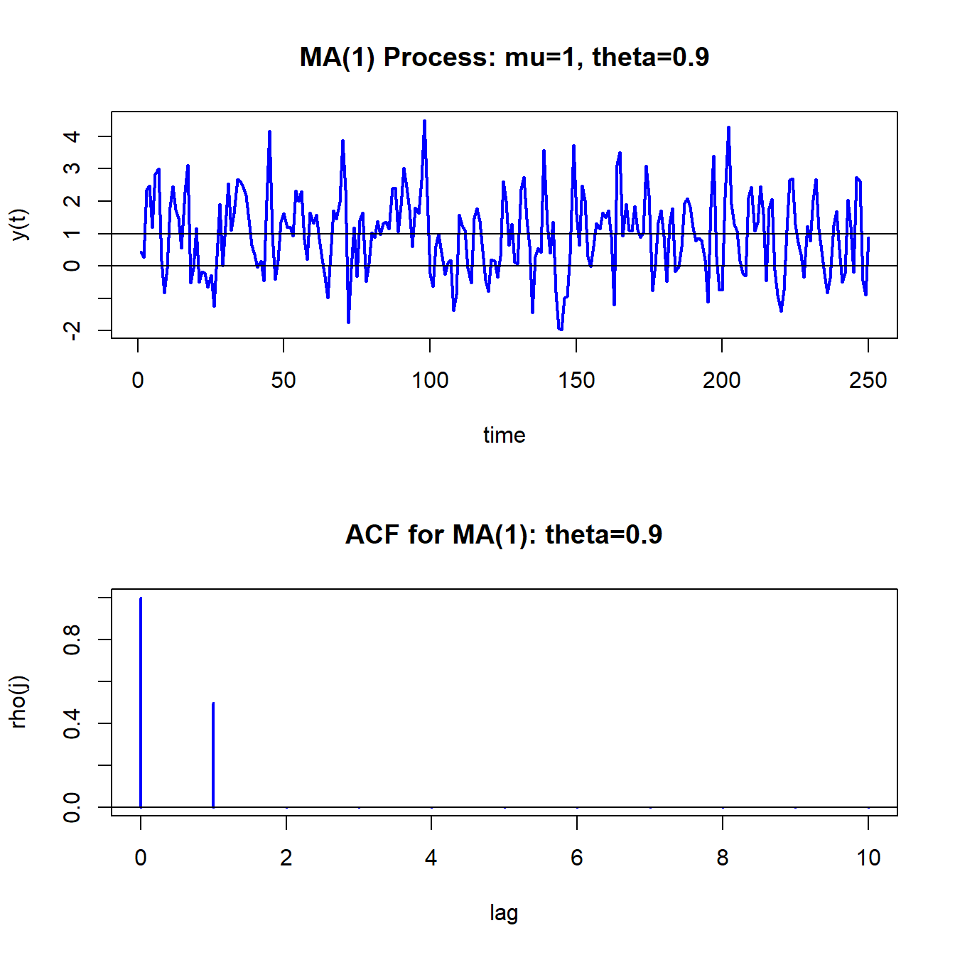
Figure 4.8: Simulated values and theoretical ACF from MA(1) process with \(\mu=1\), \(\theta=0.9\) and \(\sigma_{\varepsilon}^{2}=1\).
Compared to the GWN process in 4.2, the MA(1) process is a bit smoother in its appearance. This is due to the positive one-period time dependence captured by \(\rho_{1}=0.4972\).
\(\blacksquare\)
Let \(R_{t}\) denote the one-month continuously compounded return and assume that: \[ R_{t}\sim ~\mathrm{GWN}(\mu,\sigma^{2}). \] Consider creating a monthly time series of two-month continuously compounded returns using: \[ R_{t}(2)=R_{t}+R_{t-1}. \] The time series of these two-month returns, observed monthly, overlap by one month: \[\begin{align*} R_{t}(2) & =R_{t}+R_{t-1},\\ R_{t-1}(2) & =R_{t-1}+R_{t-2},\\ R_{t-2}(2) & =R_{t-2}+R_{t-3},\\ & \vdots \end{align*}\] The one-month overlap in the two-month returns implies that \(\{R_{t}(2)\}\) follows an MA(1) process. To show this, we need to show that the autocovariances of \(\{R_{t}(2)\}\) behave like the autocovariances of an MA(1) process.
To verify that \(\{R_{t}(2)\}\) follows an MA(1) process, first we have: \[\begin{align*} E[R_{t}(2)] & =E[R_{t}]+E[R_{t-1}]=2\mu,\\ \mathrm{var}(R_{t}(2)) & =\mathrm{var}(R_{t}+R_{t-1})=2\sigma^{2}. \end{align*}\] Next, we have: \[ \mathrm{cov}(R_{t}(2),R_{t-1}(2))=\mathrm{cov}(R_{t}+R_{t-1},R_{t-1}+R_{t-2})=\mathrm{cov}(R_{t-1},R_{t-1})=\mathrm{var}(R_{t-1})=\sigma^{2}, \] and, \[\begin{align*} \mathrm{cov}(R_{t}(2),R_{t-2}(2)) & =\mathrm{cov}(R_{t}+R_{t-1},R_{t-2}+R_{t-3})=0,\\ \mathrm{cov}(R_{t}(2),R_{t-j}(2)) & =0\text{ for }j>1. \end{align*}\] Hence, the autocovariances of \(\{R_{t}(2)\}\) are those of an MA(1) process.
Notice that \[ \rho_{1}=\frac{\sigma^{2}}{2\sigma^{2}}=\frac{1}{2}. \] What MA(1) process describes \(\{R_{t}(2)\}\)? Because \(\rho_{1}=\frac{\theta}{1+\theta^{2}}=0.5\) it follows that \(\theta=1\). Hence, the MA(1) process has mean \(2\mu\) and \(\theta=1\) and can be expressed as the MA(1) model: \[\begin{align*} R_{t}(2) & =2\mu+\varepsilon_{t}+\varepsilon_{t-1},\\ & \varepsilon_{t}\sim\mathrm{GWN}(0,\sigma^{2}). \end{align*}\]
Notice that this is a non-invertible MA(1) model.
\(\blacksquare\)
4.3.1.2 MA(q) Model
The MA(\(q\)) model has the form \[\begin{equation} Y_{t}=\mu+\varepsilon_{t}+\theta_{1}\varepsilon_{t-1}+\cdots+\theta_{q}\varepsilon_{t-q},\text{ where }\varepsilon_{t}\sim\mathrm{GWN}(0,\sigma_{\varepsilon}^{2}).\tag{4.3} \end{equation}\] The MA(q) model is stationary and ergodic provided \(\theta_{1},\ldots,\theta_{q}\) are finite. The moments of the MA(\(q\)) (see end-of-chapter exercises) are \[\begin{align*} E[Y_{t}] & =\mu,\\ \gamma_{0} & =\sigma^{2}(1+\theta_{1}^{2}+\cdots+\theta_{q}^{2}),\\ \gamma_{j} & =\left\{ \begin{array}{c} \left(\theta_{j}+\theta_{j+1}\theta_{1}+\theta_{j+2}\theta_{2}+\cdots+\theta_{q}\theta_{q-j}\right)\sigma^{2}\text{ for }j=1,2,\ldots,q\\ 0\text{ for }j>q \end{array}.\right. \end{align*}\] Hence, the ACF of an MA(\(q\)) is non-zero up to lag \(q\) and is zero afterward.
MA(\(q\)) models often arise in finance through data aggregation transformations. For example, let \(R_{t}=\ln(P_{t}/P_{t-1})\) denote the monthly continuously compounded return on an asset with price \(P_{t}\). Define the annual return at time \(t\) using monthly returns as \(R_{t}(12)=\ln(P_{t}/P_{t-12})=\sum_{j=0}^{11}R_{t-j}\). Suppose \(R_{t}\sim\mathrm{GWN}(\mu,\sigma^{2})\) and consider a sample of monthly returns of size \(T\), \(\{R_{1},R_{2},\ldots,R_{T}\}\). A sample of annual returns may be created using overlapping or non-overlapping returns. Let \(\{R_{12}(12),R_{13}(12),\) \(\ldots,R_{T}(12)\}\) denote a sample of \(T^{\ast}=T-11\) monthly overlapping annual returns and \(\{R_{12}(12),R_{24}(12),\ldots,R_{T}(12)\}\) denote a sample of \(T/12\) non-overlapping annual returns. Researchers often use overlapping returns in analysis due to the apparent larger sample size. One must be careful using overlapping returns because the monthly annual return sequence \(\{R_{t}(12)\}\) is not a Gaussian white noise process even if the monthly return sequence \(\{R_{t}\}\) is. To see this, straightforward calculations give: \[\begin{eqnarray*} E[R_{t}(12)] & = & 12\mu,\\ \gamma_{0} & = & \mathrm{var}(R_{t}(12))=12\sigma^{2},\\ \gamma_{j} & = & \mathrm{cov}(R_{t}(12),R_{t-j}(12))=(12-j)\sigma^{2}\text{ for }j<12,\\ \gamma_{j} & = & 0\text{ for }j\geq12. \end{eqnarray*}\] Since \(\gamma_{j}=0\) for \(j\geq12\) notice that \(\{R_{t}(12)\}\) behaves like an MA(11) process: \[\begin{eqnarray*} R_{t}(12) & = & 12\mu+\varepsilon_{t}+\theta_{1}\varepsilon_{t-1}+\cdots+\theta_{11}\varepsilon_{t-11},\\ \varepsilon_{t} & \sim & \mathrm{GWN}(0,\sigma^{2}). \end{eqnarray*}\]
\(\blacksquare\)
4.3.2 Autoregressive Models
Moving average models can capture almost any kind of autocorrelation structure. However, this may require many moving average terms in (4.3). Another type of simple time series model is the autoregressive model. This model can capture complex autocorrelation patterns with a small number of parameters and is used more often in practice than the moving average model.
4.3.2.1 AR(1) Model
Suppose you want to create a covariance stationary and ergodic stochastic process \(\{Y_{t}\}\) in which \(Y_{t}\) and \(Y_{t-1}\) are correlated, \(Y_{t}\) and \(Y_{t-2}\) are slightly less correlated, \(Y_{t}\) and \(Y_{t-3}\) are even less correlated and eventually \(Y_{t}\) and \(Y_{t-j}\) are uncorrelated for \(j\) large enough. That is, the time dependence in the process decays to zero as the random variables in the process get farther and farther apart. Such a process can be created using the first order autoregressive (AR(1)) model: \[\begin{align} Y_{t}-\mu & =\phi(Y_{t-1}-\mu)+\varepsilon_{t},~-1<\phi<1\tag{4.4}\\ & \varepsilon_{t}\sim\mathrm{iid}~N(0,\sigma_{\varepsilon}^{2})\nonumber \end{align}\] It can be shown that the AR(1) model is covariance stationary and ergodic provided \(-1<\phi<1\). We will show that the AR(1) process has the following properties: \[\begin{align} E[Y_{t}] & =\mu,\tag{4.5}\\ \mathrm{var}(Y_{t}) & =\sigma^{2}=\sigma_{\varepsilon}^{2}/(1-\phi^{2}),\tag{4.6}\\ \mathrm{cov}(Y_{t},Y_{t-1}) & =\gamma_{1}=\sigma^{2}\phi,\tag{4.7}\\ \mathrm{cor}(Y_{t},Y_{t-1}) & =\rho_{1}=\gamma_{1}/\sigma^{2}=\phi,\tag{4.8}\\ \mathrm{cov}(Y_{t},Y_{t-j}) & =\gamma_{j}=\sigma^{2}\phi^{j},\tag{4.9}\\ \mathrm{cor}(Y_{t},Y_{t-j}) & =\rho_{j}=\gamma_{j}/\sigma^{2}=\phi^{j}.\tag{4.10} \end{align}\] Notice that the restriction \(|\phi|<1\) implies that: \[ \lim_{j\rightarrow\infty}\rho_{j}=\phi^{j}=0, \] so that \(Y_{t}\) is essentially independent of \(Y_{t-j}\) for large \(j\) and so \(\{Y_{t}\}\) is ergodic\(.\) For example, if \(\phi=0.5\) then \(\rho_{10}=(0.5)^{10}=0.001\); if \(\phi=0.9\) then \(\rho_{10}=(0.9)^{10}=0.349\). Hence, the closer \(\phi\) is to unity the stronger is the time dependence in the process. If \(\phi=1\), then (4.4) becomes the random walk model \(Y_{t}=Y_{t-1}+\varepsilon_{t}\) and is a non-stationary process.
Verifying covariance stationarity for the AR(1) model is more involved than for the MA(1) model, and establishing the properties (4.5) - (4.10) involves some tricks. In what follows, we will assume that \(\{Y_{t}\}\) is a covariance stationary process and that \(|\phi|<1.\) First, consider the derivation for (4.5). We have: \[\begin{align*} E[Y_{t}] & =\mu+\phi(E[Y_{t-1}]-\mu)+E[\varepsilon_{t}]\\ & =\mu+\phi E[Y_{t-1}]-\phi\mu. \end{align*}\] Here, we use the first trick. Given that \(\{Y_{t}\}\) is covariance stationary it follows that \(E[Y_{t}]=E[Y_{t-1}].\) Substituting \(E[Y_{t}]=E[Y_{t-1}]\) into the above and solving for \(E[Y_{t}]\) gives (4.5).
A similar trick can be used to derive (4.6): \[ \mathrm{var}(Y_{t})=\phi^{2}(\mathrm{var}(Y_{t-1}))+\mathrm{var}(\varepsilon_{t})=\phi^{2}(\mathrm{var}(Y_{t}))+\sigma_{\varepsilon}^{2}, \] which uses the fact that \(Y_{t-1}\) is independent of \(\varepsilon_{t}\) (because \(Y_{t-1}\) only depends on \(t-1\) values) and \(\mathrm{var}(Y_{t})=\mathrm{var}(Y_{t-1})\) given that \(\{Y_{t}\}\) is covariance stationary. Solving for \(\sigma^{2}=\mathrm{var}(Y_{t})\) gives (4.6).
To determine (4.7), we use another trick. Multiply both sides of (4.4) by \(Y_{t-1}-\mu\) and take expectations to give: \[ \gamma_{1}=E\left[\left(Y_{t}-\mu\right)\left(Y_{t-1}-\mu\right)\right]=\phi E\left[(Y_{t-1}-\mu)^{2}\right]+E\left[\varepsilon_{t}\left(Y_{t-1}-\mu\right)\right]=\phi\sigma^{2}, \] which uses the fact that \(Y_{t-1}\) is independent of \(\varepsilon_{t}\), and \(\mathrm{var}(Y_{t})=\mathrm{var}(Y_{t-1})=\sigma^{2}\). Finally, to determine (4.9), multiply both sides of (4.4) by \(Y_{t-j}-\mu\) and take expectations to give: \[\begin{align*} \gamma_{j} & =E\left[\left(Y_{t}-\mu\right)\left(Y_{t-j}-\mu\right)\right]=\phi E\left[(Y_{t-1}-\mu)(Y_{t-j}-\mu)\right]+E\left[\varepsilon_{t}\left(Y_{t-j}-\mu\right)\right]\\ & =\phi\gamma_{j-1}, \end{align*}\] which uses the fact that \(Y_{t-j}\) is independent of \(\varepsilon_{t}\), and \(E\left[(Y_{t-1}-\mu)(Y_{t-j}-\mu)\right]=\gamma_{j-1}\) provided \(\{Y_{t}\}\) is covariance stationary. Using recursive substitution and \(\gamma_{0}=\sigma^{2}\) gives (4.9).
The AR(1) model (4.4) is written in what is called the mean-adjusted form. The mean-adjusted form can be re-expressed in the form of a linear regression model as follows: \[\begin{align} Y_{t}-\mu & =\phi(Y_{t-1}-\mu)+\varepsilon_{t}\Rightarrow\\ Y_{t} & =\mu-\phi\mu+\phi Y_{t-1}+\varepsilon_{t}\\ & =c+\phi Y_{t-1}+\varepsilon_{t},\tag{4.11} \end{align}\] where \(c=(1-\phi)\mu\Rightarrow\mu=c/(1-\phi)\) is the intercept of the linear regression. This regression model form is convenient for estimation by ordinary least squares.
Consider simulating 250 observations from (4.4) with \(\mu=1\), \(\phi=0.9\) and \(\sigma_{\varepsilon}=1\). To start the simulation, an initial value or start-up value for \(Y_{0}\) is required. A commonly used initial value is the mean value \(\mu\) so that \(Y_{1}=\mu+\varepsilon_{1}.\) As with the MA(1) model, this can be performed using a simple “for loop” in R:
phi = 0.9
mu = 1
sigma.e = 1
n.obs = 250
y = rep(0, n.obs)
set.seed(123)
e = rnorm(n.obs, sd=sigma.e)
y[1] = mu + e[1]
for (i in 2:n.obs) {
     y[i] = mu + phi*(y[i-1] - mu) + e[i]
}
head(y, 3)
## [1] 0.4395244 0.2653944 1.8975633Unfortunately, there is no easy way to vectorize the loop calculation.
However, the R function filter(), with optional argument
method = "recursive", implements the AR(1) recursion
efficiently in C code and so is more efficient than the for loop code
in R above:
## [1] 0.4395244 0.2653944 1.8975633The R function arima.sim(), which internally uses the filter()
function, can also be used to simulate observations from an AR(1)
process. For the AR(1) model, the function arima.sim() simulates
the components form of the AR(1) model
\[\begin{eqnarray*}
Y_{t} & = & \mu+u_{t,}\\
u_{t} & = & \phi u_{t-1}+\epsilon_{t}.
\end{eqnarray*}\]
Hence, to replicate the “for loop” simulation with arima.sim()
use:
ar1.model = list(ar=0.9)
mu = 1
set.seed(123)
y = mu + arima.sim(model=ar1.model,n=250,n.start=1, start.innov=0)
head(y, 3)
## [1] 0.4395244 0.2653944 1.8975633The R function ARMAacf() can be used to compute the theoretical
ACF for an AR(1) model as follows
The simulated AR(1) values and the ACF are shown in Figure 4.9. Compared to the MA(1) process in Figure 4.8, the realizations from the AR(1) process are much smoother. That is, when \(Y_{t}\) wanders high above its mean it tends to stay above the mean for a while and when it wanders low below the mean it tends to stay below for a while.
\(\blacksquare\)
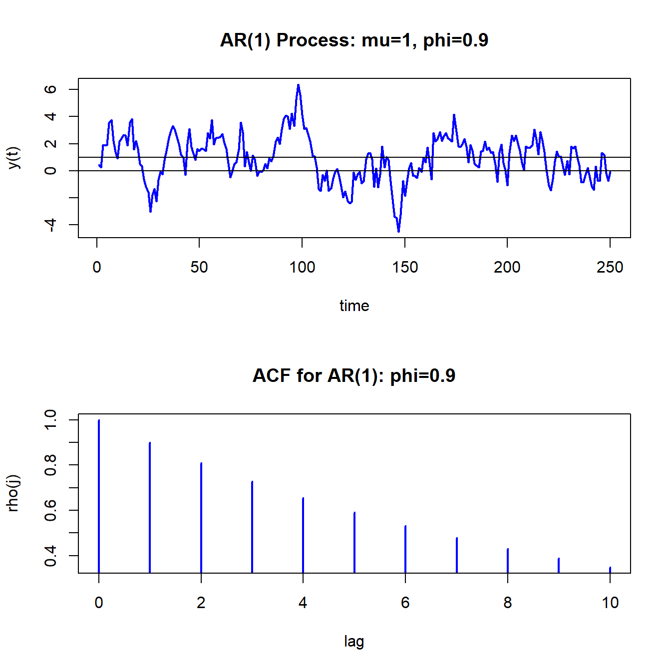
Figure 4.9: Simulated values and ACF from AR(1) model with \(\mu=1,\phi=0.9\) and \(\sigma_{\varepsilon}^{2}=1\)
- insert example showing AR(1) models with different values of \(\rho\)
- discuss the concept of mean reversion
- discuss RW model as special case of AR(1)
\(\blacksquare\)
4.3.2.2 AR(p) Model
The covariance stationary AR(\(p\)) model in mean-adjusted form is \[\begin{align} Y_{t}-\mu & =\phi_{1}(Y_{t-1}-\mu)+\cdots+\phi_{p}(Y_{t-p}-\mu)+\varepsilon_{t},\tag{4.12}\\ & \varepsilon_{t}\sim\mathrm{GWN}(0,\sigma_{\varepsilon}^{2}),\nonumber \end{align}\] where \(\mu=E[Y_{t}].\) Like the AR(1), restrictions on the autoregressive parameters \(\phi_{1},\ldots,\phi_{p}\) are required for \(\{Y_{t}\}\) to be covariance stationary and ergodic. A detailed treatment of these restrictions is beyond the scope of this book. However, one simple necessary condition for \(\{Y_{t}\}\) to be covariance stationary is \(|\phi|<1\) where \(\phi=\phi_{1}+\cdots+\phi_{p}.\) Hence, in the AR(p) model the sum of the autoregressive components \(\phi\) has a similar interpretation as the single autoregressive coefficient in the AR(1) model.
The regression form of the AR(p) is \[ Y_{t}=c+\phi_{1}Y_{t-1}+\cdots+\phi_{p}Y_{t-p}+\varepsilon_{t}, \] where \(c=\mu/(1-\phi_{1}-\cdots-\phi_{p})=\mu/(1-\phi).\) This form is convenient for estimation purposes because it is in the form of a linear regression.
The regression form of the AR(p) model is used very often in practice because of its simple linear structure and because it can capture a wide variety of autocorrelation patterns such as exponential decay, damped cyclical patterns, and oscillating damped cyclical patterns. Unfortunately, the mathematical derivation of the autocorrelations in the AR(p) model is complicated and tedious (and beyond the scope of this book). The exercises at the end of the chapter illustrate some of the calculations for the AR(2) model.
4.3.3 Autoregressive Moving Average Models
Autoregressive and moving average models can be combined into a general model called the autoregressive moving average (ARMA) model. The ARMA model with \(p\) autoregressive components and \(q\) moving average components, denoted ARMA(p,q) is given by \[\begin{align} Y_{t}-\mu & =\phi_{1}(Y_{t-1}-\mu)+\cdots+\phi_{p}(Y_{t-p}-\mu) \nonumber \\ & +\varepsilon_{t}+\theta_{1}\varepsilon_{t-1}+\cdots+\theta_{q}\varepsilon_{t-q} \tag{4.13} \\ \varepsilon_{t} & \sim\mathrm{GWN}(0,\sigma^{2}) \nonumber \end{align}\] The regression formulation is \[ Y_{t}=c+\phi_{1}Y_{t-1}+\cdots+\phi_{p}Y_{t-p}+\varepsilon_{t}+\theta\varepsilon_{t-1}+\cdots+\theta\varepsilon_{t-q} \] where \(c=\mu/(1-\phi_{1}-\cdots-\phi_{p})=\mu/(1-\phi)\) and \(\phi=\phi_{1}+\cdots+\phi_{p}.\) This model combines aspects of the pure moving average models and the pure autoregressive models and can capture many types of autocorrelation patterns. For modeling typical non-seasonal economic and financial data, it is seldom necessary to consider models in which \(p>2\) and \(q>2\). For example, the simple ARMA(1,1) model
\[\begin{equation} Y_{t}-\mu = \phi_{1}(Y_{t-1}-\mu) + \varepsilon_{t}+\theta_{1}\varepsilon_{t-1} \tag{4.14} \end{equation}\]
can capture many realistic autocorrelations observed in data.
4.3.4 Vector Autoregressive Models
The most popular multivariate time series model is the (VAR) model. The VAR model is a multivariate extension of the univariate autoregressive model (4.12). For example, a bivariate VAR(1) model for \(\mathbf{Y}_{t}=(Y_{1t},Y_{2t})^{\prime}\) has the form \[ \left(\begin{array}{c} Y_{1t}\\ Y_{2t} \end{array}\right)=\left(\begin{array}{c} c_{1}\\ c_{2} \end{array}\right)+\left(\begin{array}{cc} a_{11}^{1} & a_{12}^{1}\\ a_{21}^{1} & a_{22}^{1} \end{array}\right)\left(\begin{array}{c} Y_{1t-1}\\ Y_{2t-1} \end{array}\right)+\left(\begin{array}{c} \varepsilon_{1t}\\ \varepsilon_{2t} \end{array}\right), \] or \[\begin{align*} Y_{1t} & =c_{1}+a_{11}^{1}Y_{1t-1}+a_{12}^{1}Y_{2t-1}+\varepsilon_{1t},\\ Y_{2t} & =c_{2}+a_{21}^{1}Y_{1t-1}+a_{22}^{1}Y_{2t-1}+\varepsilon_{2t}, \end{align*}\] where \[ \left(\begin{array}{c} \varepsilon_{1t}\\ \varepsilon_{2t} \end{array}\right)\sim\mathrm{iid}\text{ }N\left(\left(\begin{array}{c} 0\\ 0 \end{array}\right),\left(\begin{array}{cc} \sigma_{11} & \sigma_{12}\\ \sigma_{12} & \sigma_{22} \end{array}\right)\right). \] In the equations for \(Y_{1}\) and \(Y_{2}\), the lagged values of both \(Y_{1}\) and \(Y_{2}\) are present. Hence, the VAR(1) model allows for dynamic feedback between \(Y_{1}\) and \(Y_{2}\) and can capture cross-lag correlations between the variables. In matrix notation, the model is \[\begin{eqnarray*} \mathbf{Y}_{t} & = & \mathbf{A}\mathbf{Y}_{t-1}+\mathbf{\varepsilon}_{t},\\ \mathbf{\varepsilon}_{t} & \sim & N(\mathbf{0},\,\Sigma), \end{eqnarray*}\] where \[ \mathbf{A}=\left(\begin{array}{cc} a_{11}^{1} & a_{12}^{1}\\ a_{21}^{1} & a_{22}^{1} \end{array}\right),\,\Sigma=\left(\begin{array}{cc} \sigma_{11} & \sigma_{12}\\ \sigma_{12} & \sigma_{22} \end{array}\right). \]
The general VAR(\(p\)) model for \(\mathbf{Y}_{t}=(Y_{1t},Y_{2t},\ldots,Y_{nt})^{\prime}\) has the form \[ \mathbf{Y}_{t}=\mathbf{c+A}_{1}\mathbf{Y}_{t-1}+\mathbf{A}_{2}\mathbf{Y}_{t-2}+\cdots+\mathbf{A}_{p}\mathbf{Y}_{t-p}+\mathbf{\varepsilon}_{t}, \] where \(\mathbf{A}_{i}\) are \((n\times n)\) coefficient matrices and \(\mathbf{\varepsilon}_{t}\) is an \((n\times1)\) unobservable zero mean white noise vector process with covariance matrix \(\Sigma\). VAR models are capable of capturing much of the complicated dynamics observed in stationary multivariate time series.
To be completed
References
Box, G., and G. M. Jenkins. 1976. Time Series Analysis : Forecasting and Control. San Francisco: Holden-Day.
Sims, C. A. 1980. Macroeconomics and Reality. Econometrica.