13.4 Quadratic Programming Problems

In this Section, we show that the inequality constrained portfolio optimization problems (13.2) and (13.3) are special cases of more general quadratic programming problems and we show how to use the function solve.QP() from the R package quadprog to numerically solve these problems.

Quadratic programming (QP) problems are of the form: \[\begin{align} \min_{\mathbf{x}}&\text{ }\frac{1}{2}\mathbf{x}^{\prime}\mathbf{Dx}-\mathbf{d}^{\prime}\mathbf{x},\tag{13.4}\\ \text{s.t. }& \mathbf{A}_{eq}^{\prime}\mathbf{x} \geq\mathbf{b}_{eq}\text{ for }l\text{ equality constraints,}\tag{13.5}\\ & \mathbf{A}_{neq}^{\prime}\mathbf{x} =\mathbf{b}_{neq}\text{ for }m\text{ inequality constraints},\tag{13.6} \end{align}\] where \(\mathbf{D}\) is an \(N\times N\) matrix, \(\mathbf{x}\) and \(\mathbf{d}\) are \(N\times1\) vectors, \(\mathbf{A}_{neq}^{\prime}\) is an \(m\times N\) matrix, \(\mathbf{b}_{neq}\) is an \(m\times1\) vector, \(\mathbf{A}_{eq}^{\prime}\) is an \(l\times N\) matrix, and \(\mathbf{b}_{eq}\) is an \(l\times1\) vector.

The solve.QP() function from the R package quadprog can be used to solve QP functions of the form (13.4) - (13.6). The function solve.QP() takes as input the matrices and vectors \(\mathbf{D}\), \(\mathbf{d}\), \(\mathbf{A}_{eq}\), \(\mathbf{b}_{eq},\) \(\mathbf{A}_{neq}\) and \(\mathbf{b}_{neq}\):

library(quadprog)
args(solve.QP)

## function (Dmat, dvec, Amat, bvec, meq = 0, factorized = FALSE) 
## NULL

where the arguments Dmat and dvec correspond to the matrix \(\mathbf{D}\) and the vector \(\mathbf{d}\), respectively. The function solve.QP(), however, assumes that the equality and inequality matrices (\(\mathbf{A}_{eq},\,\mathbf{A}_{neq}\)) and vectors (\(\mathbf{b}_{eq},\,\mathbf{b}_{neq}\)) are combined into a single \((l+m)\times N\) matrix \(\mathbf{A}^{\prime}\) and a single \((l+m)\)\(\times1\) vector \(\mathbf{b}\) of the form: \[ \mathbf{A}^{\prime}=\left[\begin{array}{c} \mathbf{A}_{eq}^{\prime}\\ \mathbf{A}_{neq}^{\prime} \end{array}\right],\,\mathbf{b}=\left(\begin{array}{c} \mathbf{b}_{eq}\\ \mathbf{b}_{neq} \end{array}\right). \] In solve.QP(), the argument Amat represents the matrix \(\mathbf{A}\) (not \(\mathbf{A}^{\prime})\) and the argument bmat represents the vector \(\mathbf{b}\). The argument meq determines the number of linear equality constraints (i.e., the number of rows \(l\) of \(\mathbf{A}_{eq}^{\prime}\)) so that \(\mathbf{A}^{\prime}\) can be separated into \(\mathbf{A}_{eq}^{\prime}\) and \(\mathbf{A}_{neq}^{\prime}\), respectively.

13.4.1 No short sales global minimum variance portfolio

The portfolio optimization problems (13.2) and (13.3) are special cases of the general QP problem (13.4) - (13.6). Consider first the problem to find the global minimum variance portfolio (13.2). The objective function \(\sigma_{p,m}^{2}=\mathbf{m}^{\prime}\Sigma \mathbf{m}\) can be recovered from (13.4) by setting \(\mathbf{x}=\mathbf{m}\), \(\mathbf{D}=2\times\mathbf{\varSigma}\) and \(\mathbf{d}=(0,\ldots,0)^{\prime}.\) Then, \[ \frac{1}{2}\mathbf{x}^{\prime}\mathbf{Dx}-\mathbf{d}^{\prime}\mathbf{x}=\mathbf{m^{\prime}\varSigma m}=\sigma_{p,m}^{2}. \] Here, there is one equality constraint, \(\mathbf{m}^{\prime}\mathbf{1}=1\), and \(N\) inequality constraints, \(m_{i}\geq0\text{ }(i=1,\ldots,N)\), which can be expressed compactly as \(\mathbf{m}\geq\mathbf{0}\). These constraints can be expressed in the form (13.5) and (13.6) by defining the restriction matrices: \[\begin{align*} \underset{(1\times N)}{\mathbf{A}_{eq}^{\prime}} & =\mathbf{1}^{\prime},\text{ }\underset{(1\times1)}{\mathbf{b}_{eq}}=1\\ \underset{(N\times N)}{\mathbf{A}_{neq}^{\prime}} & =\mathbf{I}_{N},\underset{(N\times1)}{\mathbf{b}_{neq}}=(0,\ldots,0)^{\prime}=\mathbf{0}, \end{align*}\] so that \[ \mathbf{A}^{\prime}=\left[\begin{array}{c} \mathbf{1}^{\prime}\\ \mathbf{I}_{N} \end{array}\right],\,\mathbf{b}=\left(\begin{array}{c} 1\\ \mathbf{0} \end{array}\right). \] Here, \[\begin{eqnarray*} \mathbf{A}_{eq}^{\prime}\mathbf{m} & = & \mathbf{1^{\prime}m}=1=b_{eq},\\ \mathbf{A}_{neq}^{\prime}\mathbf{m} & = & \mathbf{I}_{N}\mathbf{m}=\mathbf{m}\geq\mathbf{0}=\mathbf{b}_{neq}. \end{eqnarray*}\]

Example 2.11 (Global minimum variance portfolio with no short sales for three asset example data)

The unconstrained global minimum variance portfolio of Microsoft, Nordstrom and Starbucks is:

library(IntroCompFinR)
gmin.port = globalMin.portfolio(mu.vec, sigma.mat) 
gmin.port

## Call:
## globalMin.portfolio(er = mu.vec, cov.mat = sigma.mat)
## 
## Portfolio expected return:     0.0249 
## Portfolio standard deviation:  0.0727 
## Portfolio weights:
##  MSFT  NORD  SBUX 
## 0.441 0.366 0.193

This portfolio does not have any negative weights and so the no-short sales restriction is not binding. Hence, the short sales constrained global minimum variance is the same as the unconstrained global minimum variance portfolio.

The restriction matrices and vectors required by solve.QP() to compute the short sales constrained global minimum variance portfolio are:

D.mat = 2*sigma.mat 
d.vec = rep(0, 3) 
A.mat = cbind(rep(1,3), diag(3)) 
b.vec = c(1, rep(0,3))
D.mat

##        MSFT   NORD   SBUX
## MSFT 0.0200 0.0036 0.0022
## NORD 0.0036 0.0218 0.0052
## SBUX 0.0022 0.0052 0.0398

d.vec

## [1] 0 0 0

t(A.mat)

##      [,1] [,2] [,3]
## [1,]    1    1    1
## [2,]    1    0    0
## [3,]    0    1    0
## [4,]    0    0    1

b.vec

## [1] 1 0 0 0

To find the short sales constrained global minimum variance portfolio, call solve.QP() with the above inputs and set meq=1 to indicate one equality constraint:

qp.out = solve.QP(Dmat=D.mat, dvec=d.vec,                   
                  Amat=A.mat, bvec=b.vec, meq=1) 
class(qp.out)

## [1] "list"

names(qp.out)

## [1] "solution"               "value"                  "unconstrained.solution"
## [4] "iterations"             "Lagrangian"             "iact"

The returned object, qp.out, is a list with the following components:

qp.out

## $solution
## [1] 0.441 0.366 0.193
## 
## $value
## [1] 0.00528
## 
## $unconstrained.solution
## [1] 0 0 0
## 
## $iterations
## [1] 2 0
## 
## $Lagrangian
## [1] 0.0106 0.0000 0.0000 0.0000
## 
## $iact
## [1] 1

The portfolio weights are in the solution component, which match the global minimum variance weights allowing short sales, and satisfy the required constraints (weights sum to one and all weights are positive). The minimized value of the objective function (portfolio variance) is in the value component. See the help file for solve.QP() for explanations of the other components.

You can also use the IntroCompFinR function globalmin.portfolio() to compute the global minimum variance portfolio subject to short-sales constraints by specifying the optional argument shorts=FALSE:

gmin.port = globalMin.portfolio(mu.vec, sigma.mat,                                 
                                shorts=FALSE)
gmin.port

## Call:
## globalMin.portfolio(er = mu.vec, cov.mat = sigma.mat, shorts = FALSE)
## 
## Portfolio expected return:     0.0249 
## Portfolio standard deviation:  0.0727 
## Portfolio weights:
##  MSFT  NORD  SBUX 
## 0.441 0.366 0.193

When shorts=FALSE, globalmin.portfolio() uses solve.QP() as described above to do the optimization.

\(\blacksquare\)

13.4.2 No short sales minimum variance portfolio with target expected return

Next, consider the problem (13.3) to find a minimum variance portfolio with a given target expected return. The objective function (13.4) has \(\mathbf{D}=2\times\mathbf{\varSigma}\) and \(\mathbf{d}=(0,\ldots,0)^{\prime}.\) The two linear equality constraints, \(\mathbf{x}^{\prime}\mu=\mu_{p}^{0}\) and \(\mathbf{x}^{\prime}\mathbf{1}=1\), and \(N\) inequality constraints \(\mathbf{x}\geq\mathbf{0}\) have restriction matrices and vectors: \[\begin{align*} \underset{(2\times N)}{\mathbf{A}_{eq}^{\prime}} & =\left(\begin{array}{c} \mu^{\prime}\\ \mathbf{1}^{\prime} \end{array}\right),\,\underset{(2\times1)}{\mathbf{b}_{eq}}=\left(\begin{array}{c} \mu_{p}^{0}\\ 1 \end{array}\right).\text{ }\\ \underset{(N\times N)}{\mathbf{A}_{neq}^{\prime}} & =\mathbf{I}_{N},\,\underset{(N\times1)}{\mathbf{b}_{neq}}=(0,\ldots,0)^{\prime}. \end{align*}\] so that \[ \mathbf{A}^{\prime}=\left(\begin{array}{c} \mu^{\prime}\\ \mathbf{1}^{\prime}\\ \mathbf{I}_{N} \end{array}\right),\text{ }\mathbf{b}=\left(\begin{array}{c} \mu_{p}^{0}\\ 1\\ \mathbf{0} \end{array}\right). \] Here, \[\begin{eqnarray*} \mathbf{A}_{eq}^{\prime}\mathbf{x} & = & \left(\begin{array}{c} \mu^{\prime}\\ \mathbf{1}^{\prime} \end{array}\right)\mathbf{x=}\left(\begin{array}{c} \mu^{\prime}\mathbf{x}\\ \mathbf{1}^{\prime}\mathbf{x} \end{array}\right)=\left(\begin{array}{c} \mu_{p}^{0}\\ 1 \end{array}\right)=\mathbf{b}_{eq},\\ \mathbf{A}_{neq}^{\prime}\mathbf{x} & = & \mathbf{I}_{N}\mathbf{x}=\mathbf{x}\geq0. \end{eqnarray*}\]

Example 2.13 (Minimum variance portfolio with target expected return and no short sales for three asset example data)

Now, we consider finding the minimum variance portfolio that has the same mean as Microsoft but does not allow short sales. First, we find the minimum variance portfolio allowing for short sales using the IntroCompFinR function efficient.portfolio():

eMsft.port = efficient.portfolio(mu.vec, sigma.mat, 
                                 target.return = mu.vec["MSFT"])
eMsft.port

## Call:
## efficient.portfolio(er = mu.vec, cov.mat = sigma.mat, target.return = mu.vec["MSFT"])
## 
## Portfolio expected return:     0.0427 
## Portfolio standard deviation:  0.0917 
## Portfolio weights:
##    MSFT    NORD    SBUX 
##  0.8275 -0.0907  0.2633

This portfolio has a short sale (negative weight) in Nordstrom. Hence, when the short sales restriction is imposed it will be binding. Next, we set up the restriction matrices and vectors required by solve.QP() to compute the minimum variance portfolio with no-short sales:

D.mat = 2*sigma.mat 
d.vec = rep(0, 3) 
A.mat = cbind(mu.vec, rep(1,3), diag(3)) 
b.vec = c(mu.vec["MSFT"], 1, rep(0,3))
t(A.mat)

##          MSFT   NORD   SBUX
## mu.vec 0.0427 0.0015 0.0285
##        1.0000 1.0000 1.0000
##        1.0000 0.0000 0.0000
##        0.0000 1.0000 0.0000
##        0.0000 0.0000 1.0000

b.vec

##   MSFT                             
## 0.0427 1.0000 0.0000 0.0000 0.0000

Then we call solve.QP() with meq=2 to indicate two equality constraints:

qp.out = solve.QP(Dmat=D.mat, dvec=d.vec,                   
                  Amat=A.mat, bvec=b.vec, meq=2) 
names(qp.out$solution) = names(mu.vec)
round(qp.out$solution, digits=3)

## MSFT NORD SBUX 
##    1    0    0

With short sales not allowed, the minimum variance portfolio with the same mean as Microsoft is 100% invested in Microsoft. This is consistent with what we see in Figure 13.7. The volatility of this portfolio is slightly higher than the volatility of the portfolio that allows short sales:

sqrt(qp.out$value)

## [1] 0.1

eMsft.port$sd

## [1] 0.0917

You can also use the IntroCompFinR function efficient.portfolio() to compute a minimum variance portfolio with target expected return subject to short-sales constraints by specifying the optional argument shorts=FALSE:

efficient.portfolio(mu.vec, sigma.mat, 
                    target.return = mu.vec["MSFT"], shorts = FALSE)

## Call:
## efficient.portfolio(er = mu.vec, cov.mat = sigma.mat, target.return = mu.vec["MSFT"], 
##     shorts = FALSE)
## 
## Portfolio expected return:     0.0427 
## Portfolio standard deviation:  0.1 
## Portfolio weights:
## MSFT NORD SBUX 
##    1    0    0

Suppose you try to find a minimum variance portfolio with target return higher than the mean of Microsoft while imposing no short sales:

# efficient.portfolio(mu.vec, sigma.mat, 
#                     target.return = mu.vec["MSFT"]+0.01, 
#                     shorts = FALSE) 
# uncomment this line to see the results

Here, solve.QP() reports the error “constraints are inconsistent, no solution!” This agrees with what we see in Figure 13.7.

\(\blacksquare\)

Example 2.17 (Compute efficient frontier portfolios from three asset example data)

In this example we compare the efficient frontier portfolios computed with and without short sales. This can be easily done using the IntroCompFinR function efficient.frontier(). First, we compute the efficient frontier allowing short sales for target returns between the mean of the global minimum variance portfolio and the mean of Microsoft:

ef = efficient.frontier(mu.vec, sigma.mat, alpha.min=0,                           
                         alpha.max=1, nport=10) 
ef$weights

##          MSFT    NORD  SBUX
## port 1  0.441  0.3656 0.193
## port 2  0.484  0.3149 0.201
## port 3  0.527  0.2642 0.209
## port 4  0.570  0.2135 0.217
## port 5  0.613  0.1628 0.224
## port 6  0.656  0.1121 0.232
## port 7  0.699  0.0614 0.240
## port 8  0.742  0.0107 0.248
## port 9  0.785 -0.0400 0.256
## port 10 0.827 -0.0907 0.263

Here, portfolio 1 is the global minimum variance portfolio and portfolio 10 is the efficient portfolio with the same mean as Microsoft. Notice that portfolios 9 and 10 have negative weights in Nordstrom. Next, we compute the efficient frontier not allowing short sales for the same range of target returns:

ef.ns = efficient.frontier(mu.vec, sigma.mat, alpha.min=0,                           
                           alpha.max=1, nport=10, shorts=FALSE) 
ef.ns$weights

##          MSFT   NORD  SBUX
## port 1  0.441 0.3656 0.193
## port 2  0.484 0.3149 0.201
## port 3  0.527 0.2642 0.209
## port 4  0.570 0.2135 0.217
## port 5  0.613 0.1628 0.224
## port 6  0.656 0.1121 0.232
## port 7  0.699 0.0614 0.240
## port 8  0.742 0.0107 0.248
## port 9  0.861 0.0000 0.139
## port 10 1.000 0.0000 0.000

Portfolios 1 - 8 have all positive weights and are the same as portfolios 1 - 8 when short sales are allowed. However, for portfolios 9 and 10 the short sales constraint is binding. For portfolio 9, the weight in Nordstrom is forced to zero and the weight in Starbucks is reduced. For portfolio 10, the weights on Nordstrom and Starbucks are forced to zero. The two frontiers are illustrated in Figure 13.8. For portfolios 1-8, the two frontiers coincide. For portfolios 9 and 10, the no-shorts frontier lies inside and to the right of the short-sales frontier. The cost of the short sales constraint is the increase in the volatility of minimum variance portfolios for target returns near the expected return on Microsoft.

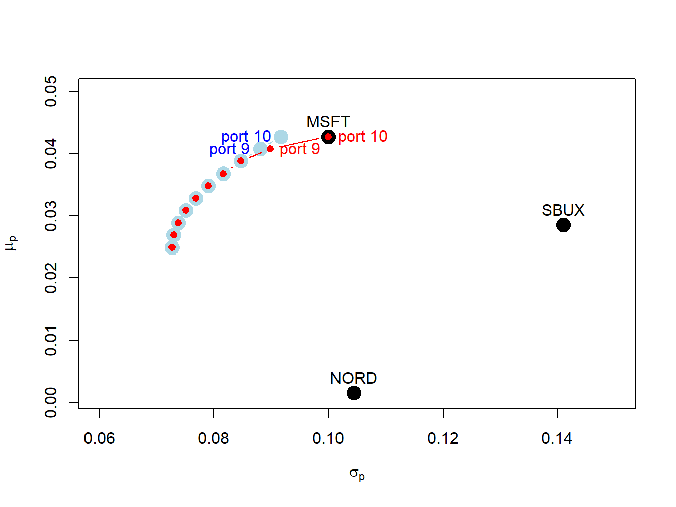
Efficient frontier portfolios with and without short sales. The unconstrained efficient frontier portfolios are in blue, and the short sales constrained efficient portfolios are in red. The unconstrained portfolios labeled "port 9" and "port 10" have short sales in Nordstrom. The constrained portfolio labeled "port 9" has zero weight in Nordstrom, and the constrained portfolio labeled "port 10align has zero weights in Nordstrom and Starbucks.

Figure 13.8: Efficient frontier portfolios with and without short sales. The unconstrained efficient frontier portfolios are in blue, and the short sales constrained efficient portfolios are in red. The unconstrained portfolios labeled “port 9” and “port 10” have short sales in Nordstrom. The constrained portfolio labeled “port 9” has zero weight in Nordstrom, and the constrained portfolio labeled "port 10align has zero weights in Nordstrom and Starbucks.

13.4.3 No short sales tangency portfolio

Consider an investment universe with \(N\) risky assets and a single risk-free asset. We assume that short sales constraints only apply to the \(N\) risky assets, and that investors can borrow and lend at the risk-free rate \(r_{f}\). As shown in Chapter 12, with short sales allowed, mean-variance efficient portfolios are combinations of the risk-free asset and the tangency portfolio. The tangency portfolio is the maximum Sharpe ratio portfolio of risky assets and is the solution to the maximization problem: \[\begin{eqnarray*} \underset{\mathbf{t}}{\max}\,\frac{\mu_{t}-r_{f}}{\sigma_{t}} & = & \frac{\mathbf{t}^{\prime}\mu-r_{f}}{(\mathbf{t}^{\prime}\Sigma\mathbf{t})^{1/2}}\,s.t.\\ \mathbf{t}^{\prime}\mathbf{1} & = & 1. \end{eqnarray*}\]

Example 2.18 (Compute efficient portfolios allowing short sales from three asset example data when there is a risk-free asset)

Assuming a risk-free rate \(r_{f}=0.005\), we can compute the unconstrained tangency portfolio for the three asset example data using the IntroCompFinR function tangency.portfolio():

r.f = 0.005 
tan.port = tangency.portfolio(mu.vec, sigma.mat, r.f) 
summary(tan.port, r.f)

## Call:
## tangency.portfolio(er = mu.vec, cov.mat = sigma.mat, risk.free = r.f)
## 
## Portfolio expected return:     0.0519 
## Portfolio standard deviation:  0.112 
## Portfolio Sharpe Ratio:        0.42 
## Portfolio weights:
##   MSFT   NORD   SBUX 
##  1.027 -0.326  0.299

Here, the unconstrained tangency portfolio has a negative weight in Nordstrom so that the short sales constraint on the risky assets will be binding. The unconstrained set of efficient portfolios, that are combinations of the risk-free asset and the unconstrained tangency portfolio, is illustrated in Figure 13.9.

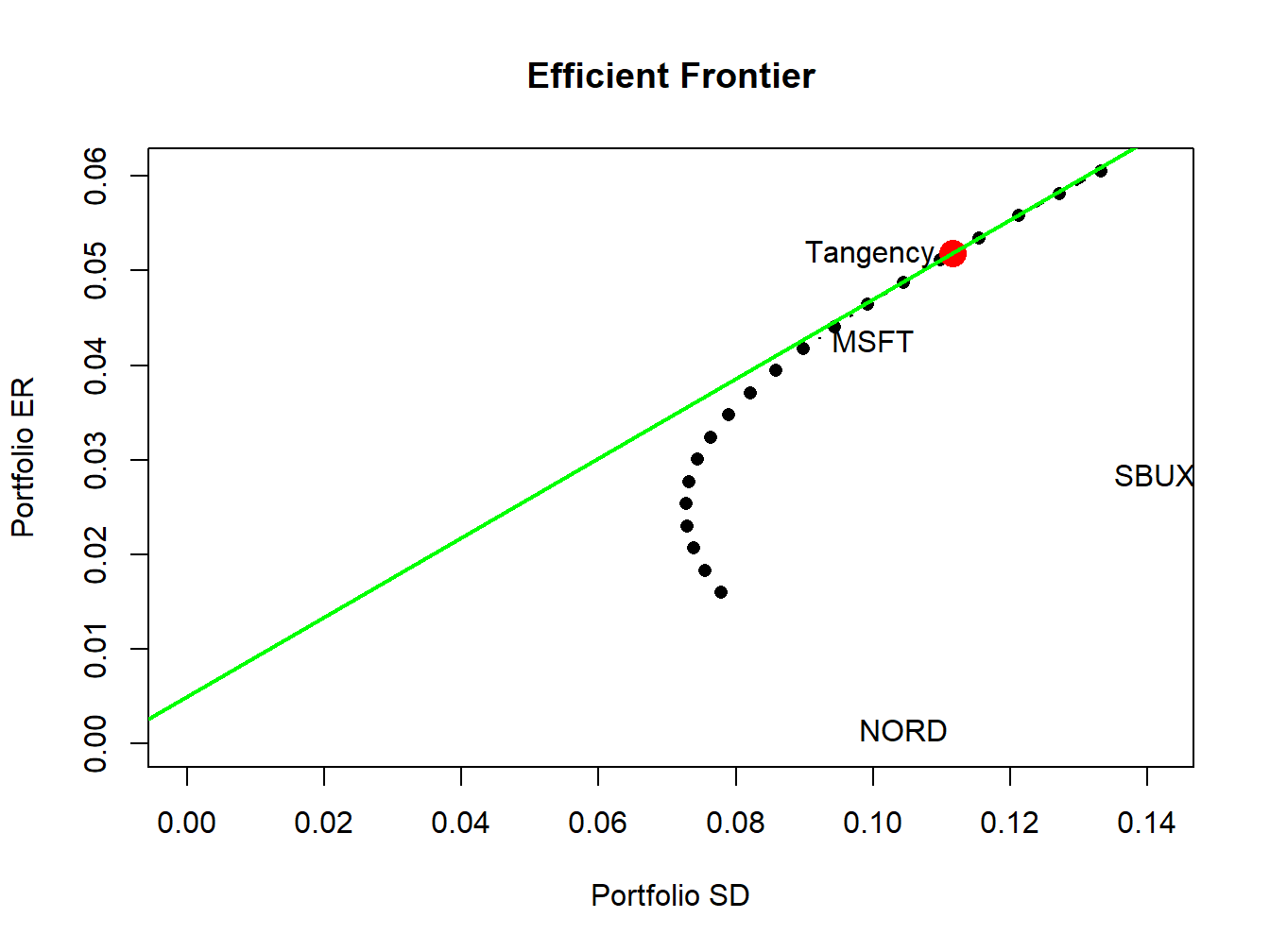
Efficient portfolios of three risky assets and a risk-free asset allowing short sales. Nordstrom is sold short in the unconstrained tangency portfolio.

Figure 13.9: Efficient portfolios of three risky assets and a risk-free asset allowing short sales. Nordstrom is sold short in the unconstrained tangency portfolio.

Here, we see that the unconstrained tangency portfolio is located on the frontier of risky asset portfolios above the point labeled “MSFT”. The green line represents portfolios of the risk-free asset and the unconstrained tangency portfolio.

\(\blacksquare\)

Under short sales constraints on the risky assets, the maximum Sharpe ratio portfolio solves: \[\begin{eqnarray*} \max_{\mathbf{t}}\,\frac{\mu_{t}-r_{f}}{\sigma_{t}} & = & \frac{\mathbf{t}^{\prime}\mu-r_{f}}{(\mathbf{t}^{\prime}\Sigma\mathbf{t})^{1/2}}\,s.t.\\ \mathbf{t}^{\prime}\mathbf{1} & = & 1,\\ t_{i} & \geq & 0,\,i=1,\ldots,N. \end{eqnarray*}\] This optimization problem cannot be written as a QP optimization as expressed in (13.4) - (13.6). Hence, it looks like we cannot use the function solve.QP() to find the short sales constrained tangency portfolio. However, it turns out we can use solve.QP() to find the short sales constrained tangency portfolio. To do this we utilize the alternative derivation of the tangency portfolio presented in Chapter 12. The alternative way to compute the tangency portfolio is to first find a minimum variance portfolio of risky assets and a risk-free asset whose excess expected return, \(\tilde{\mu}_{p,x}=\mu^{\prime}\mathbf{x}-r_{f}\mathbf{1}\), achieves a target excess return \(\tilde{\mu}_{p,0}=\mu_{p,0}-r_{f}>0\). This portfolio solves the minimization problem: \[ \min_{\mathbf{x}}~\sigma_{p,x}^{2}=\mathbf{x}^{\prime}\Sigma \mathbf{x}\textrm{ s.t. }\tilde{\mu}_{p,x}=\tilde{\mu}_{p,0}, \] where the weight vector \(\mathbf{x}\) is not constrained to satisfy \(\mathbf{x}^{\prime}\mathbf{1}=\mathbf{1}\). The tangency portfolio is then determined by normalizing the weight vector \(\mathbf{x}\) so that its elements sum to one:⁹⁰ \[ \mathbf{t}=\frac{\mathbf{x}}{\mathbf{x}^{\prime}\mathbf{1}}=\frac{\Sigma^{-1}(\mu-r_{f}\cdot\mathbf{1})}{\mathbf{1}^{\prime}\Sigma^{-1}(\mu-r_{f}\cdot\mathbf{1})}. \] An interesting feature of this result is that it does not depend on the value of the target excess return value \(\tilde{\mu}_{p,0}=\mu_{p,0}-r_{f}>0\). That is, every value of \(\tilde{\mu}_{p,0}=\mu_{p,0}-r_{f}>0\) gives the same value for the tangency portfolio.⁹¹ We can utilize this alternative derivation of the tangency portfolio to find the tangency portfolio subject to short-sales restrictions on risky assets. First we solve the short-sales constrained minimization problem: \[\begin{eqnarray} \min_{\mathbf{x}}~\sigma_{p,x}^{2} & = & \mathbf{x}^{\prime}\Sigma \mathbf{x}\textrm{ s.t. }\tag{13.7}\\ \tilde{\mu}_{p,x} & = & \tilde{\mu}_{p,0},\tag{13.8}\\ x_{i} & \geq & 0,\,i=1,\ldots,N.\tag{13.9} \end{eqnarray}\] Here we can use any value for \(\tilde{\mu}_{p,0}\) so for convenience we use \(\tilde{\mu}_{p,0}=1\). This is a QP problem with \(\mathbf{D}=2\times\mathbf{\varSigma}\) and \(\mathbf{d}=(0,\ldots,0)^{\prime}\), one linear equality constraint, \(\tilde{\mu}_{p,x}=\tilde{\mu}_{p,0},\) and \(N\) inequality constraints \(\mathbf{x}\geq\mathbf{0}\). The restriction matrices and vectors are: \[\begin{align*} \underset{(1\times N)}{\mathbf{A}_{eq}^{\prime}} & =(\mu-r_{f}1)^{\prime},\,\underset{(1\times1)}{\mathbf{b}_{eq}}=1,\text{ }\\ \underset{(N\times N)}{\mathbf{A}_{neq}^{\prime}} & =\mathbf{I}_{N},\,\underset{(N\times1)}{\mathbf{b}_{neq}}=(0,\ldots,0)^{\prime}. \end{align*}\] so that \[ \mathbf{A}^{\prime}=\left(\begin{array}{c} (\mu-r_{f}1)^{\prime}\\ \mathbf{I}_{N} \end{array}\right),\text{ }\mathbf{b}=\left(\begin{array}{c} 1\\ \mathbf{0} \end{array}\right). \] Here, \[\begin{eqnarray*} \mathbf{A}_{eq}^{\prime}\mathbf{x} & = & (\mu-r_{f}1)^{\prime}\mathbf{x=\tilde{\mu}_{p,x}}=1,\\ \mathbf{A}_{neq}^{\prime}\mathbf{x} & = & \mathbf{I}_{N}\mathbf{x}=\mathbf{x}\geq0. \end{eqnarray*}\] After solving the QP problem for \(\mathbf{x}\), we then determine the short-sales constrained tangency portfolio by normalizing the weight vector \(\mathbf{x}\) so that its elements sum to one: \[ \mathbf{t}=\frac{\mathbf{x}}{\mathbf{x}^{\prime}\mathbf{1}}. \]

Example 2.20 (Compute efficient portfolios not allowing short sales from three asset example data when there is a risk-free asset)

First, we use solve.QP() to find the short sales restricted tangency portfolio. The restriction matrices for the short sales constrained optimization (13.7) - (13.9) are:

D.mat = 2*sigma.mat 
d.vec = rep(0, 3) 
A.mat = cbind(mu.vec - rep(1, 3)*r.f, diag(3)) 
b.vec = c(1, rep(0,3))

The un-normalized portfolio \(\mathbf{x}\) is found using:

qp.out = solve.QP(Dmat=D.mat, dvec=d.vec,                   
                  Amat=A.mat, bvec=b.vec, meq=1) 
x.ns = qp.out$solution 
names(x.ns) = names(mu.vec) 
round(x.ns, digits=3)

##  MSFT  NORD  SBUX 
## 22.74  0.00  6.08

The short sales constrained tangency portfolio is then:

t.ns = x.ns/sum(x.ns) 
round(t.ns, digits=3)

##  MSFT  NORD  SBUX 
## 0.789 0.000 0.211

In this portfolio, the allocation to Nordstrom, which was negative in the unconstrained tangency portfolio, is set to zero.

To verify that the derivation of the short sales constrained tangency portfolio does not depend on \(\tilde{\mu}_{p,0}=\mu_{p,0}-r_{f}>0\), we repeat the calculations with \(\tilde{\mu}_{p,0}=0.5\) instead of \(\tilde{\mu}_{p,0}=1\):

b.vec = c(0.5, rep(0,3)) 
qp.out = solve.QP(Dmat=D.mat, dvec=d.vec,                   
                  Amat=A.mat, bvec=b.vec, meq=1) 
x.ns = qp.out$solution 
names(x.ns) = names(mu.vec) 
t.ns = x.ns/sum(x.ns) 
round(t.ns, digits=3)

##  MSFT  NORD  SBUX 
## 0.789 0.000 0.211

You can compute the short sales restricted tangency portfolio using the IntroCompFinR function tangency.portfolio() with the optional argument shorts=FALSE:

tan.port.ns = tangency.portfolio(mu.vec, sigma.mat, r.f, shorts=FALSE) 
summary(tan.port.ns, r.f)

## Call:
## tangency.portfolio(er = mu.vec, cov.mat = sigma.mat, risk.free = r.f, 
##     shorts = FALSE)
## 
## Portfolio expected return:     0.0397 
## Portfolio standard deviation:  0.0865 
## Portfolio Sharpe Ratio:        0.401 
## Portfolio weights:
##  MSFT  NORD  SBUX 
## 0.789 0.000 0.211

Notice that the Sharpe ratio on the short sales restricted tangency portfolio is slightly smaller than the Sharpe ratio on the unrestricted tangency portfolio.

The set of efficient portfolios are combinations of the risk-free asset and the short sales restricted tangency portfolio. These portfolios are illustrated in Figure 13.10, created using:

ef.ns = efficient.frontier(mu.vec, sigma.mat, alpha.min=0,
                            alpha.max=1, nport=10, shorts=FALSE) 
plot(ef.ns, plot.assets=TRUE, pch=16) 
points(tan.port.ns$sd, tan.port.ns$er, col="red", pch=16, cex=2) 
sr.tan.ns = (tan.port.ns$er - r.f)/tan.port.ns$sd 
abline(a=r.f, b=sr.tan.ns, col="green", lwd=2) 
text(tan.port$sd, tan.port$er, labels="Tangency", pos = 2)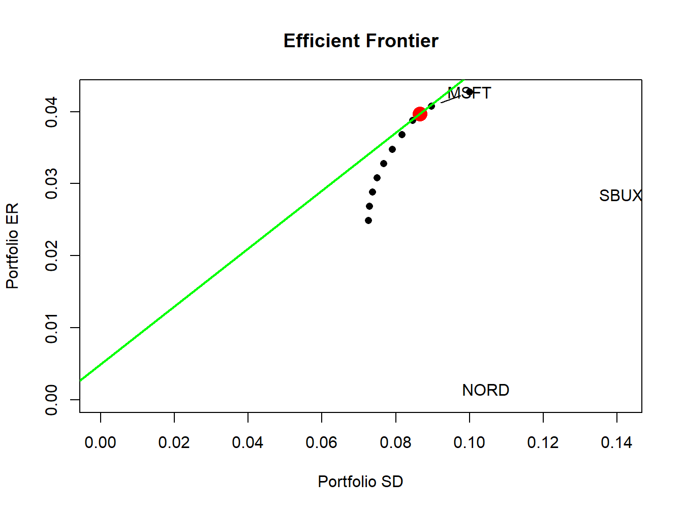

Figure 13.10: Efficient

\(\blacksquare\)

This normalization ensures that the tangency portfolio is 100% invested in the risky assets.↩︎
If \(\tilde{\mu}_{p,0}=0\) then the portfolio of risky assets and the risk-free asset has expected return equal to \(r_{f}\). In this case, \(\mathbf{x}=\mathbf{0}\) and \(x_{f}=1\). ↩︎