12.1 Portfolios with \(N\) Risky Assets
Consider a portfolio with \(N\) risky assets, where \(N\) can be a large number (e.g., \(N=1,000)\). Let \(R_{i}\) \((i=1,\ldots,N)\) denote the simple return on asset \(i\) (over some fixed time horizon such as one year) and assume that the constant expected return (GWN) model holds for all assets: \[\begin{align*} R_{i} & \sim GWN(\mu_{i},\sigma_{i}^{2}),\\ \mathrm{cov}(R_{i},R_{j}) & =\sigma_{ij}. \end{align*}\]
Let \(x_{i}\) denote the share of wealth invested in asset \(i\) \((i=1,\ldots,N)\), and assume that all wealth is invested in the \(N\) assets so that \(\sum_{i=1}^{N}x_{i}=1.\) Assume that short sales are allowed so that some values of \(x_{i}\) can be negative. The portfolio return, \(R_{p,x},\) is the random variable \(R_{p,x}=\sum_{i=1}^{N}x_{i}R_{i}.\) The subscript “\(x\)” indicates that the portfolio is constructed using the “x-weights” \(x_{1},x_{2},\ldots,x_{N}\). The expected return on the portfolio is: \[ \mu_{p,x}=\sum_{i=1}^{N}x_{i}\mu_{i}, \] and the variance of the portfolio return is: \[ \sigma_{p,x}^{2}=\sum_{i=1}^{N}x_{i}^{2}\sigma_{i}^{2}+2\sum_{i=1}^{N}\sum_{j\neq i}x_{i}x_{j}\sigma_{ij}. \] Notice that variance of the portfolio return depends on \(N\) variance terms and \(N(N-1)\) covariance terms. Hence, with \(N\) assets there are many more covariance terms than variance terms contributing to portfolio variance. For example, with \(N=100\) there are \(100\) variance terms and \(100\times99=9900\) covariance terms. With \(N\) assets, the algebra representing the portfolio return and risk characteristics is cumbersome, especially for the variance. We can greatly simplify the portfolio algebra using matrix notation, and this was previewed in Chapter 3.
12.1.1 Portfolio return and risk characteristics using matrix notation
Define the following \(N\times1\) column vectors containing the asset returns and portfolio weights: \[ \mathbf{R}=\left(\begin{array}{c} R_{1}\\ \vdots\\ R_{N} \end{array}\right),~\mathbf{x}=\left(\begin{array}{c} x_{1}\\ \vdots\\ x_{N} \end{array}\right). \] In matrix notation we can lump multiple returns in a single vector which we denote by \(\mathbf{R}\). Since each of the elements in \(\mathbf{R}\) is a random variable we call \(\mathbf{R}\) a random vector. The probability distribution of the random vector \(\mathbf{R}\) is simply the joint distribution of the elements of \(\mathbf{R}\). In the GWN model all returns are jointly normally distributed and this joint distribution is completely characterized by the means, variances and covariances of the returns. We can easily express these values using matrix notation as follows. The \(N\times1\) vector of portfolio expected values is: \[ E[\mathbf{R}]=E\left[\left(\begin{array}{c} R_{1}\\ \vdots\\ R_{N} \end{array}\right)\right]=\left(\begin{array}{c} E[R_{1}]\\ \vdots\\ E[R_{N}] \end{array}\right)=\left(\begin{array}{c} \mu_{1}\\ \vdots\\ \mu_{N} \end{array}\right)=\mu, \] and the \(N\times N\) covariance matrix of returns is:
\[\begin{align*} \mathrm{var}(\mathbf{R})& =\left(\begin{array}{cccc} \mathrm{var}(R_{1}) & \mathrm{cov}(R_{1},R_{2}) & \cdots & \mathrm{cov}(R_{1},R_{N})\\ \mathrm{cov}(R_{1},R_{2}) & \mathrm{var}(R_{2}) & \cdots & \mathrm{cov}(R_{2},R_{N})\\ \vdots & \vdots & \ddots & \vdots\\ \mathrm{cov}(R_{1},R_{N}) & \mathrm{cov}(R_{2},R_{N}) & \cdots & \mathrm{var}(R_{N}) \end{array}\right) \\ &=\left(\begin{array}{cccc} \sigma_{1}^{2} & \sigma_{12} & \cdots & \sigma_{1N}\\ \sigma_{12} & \sigma_{2}^{2} & \cdots & \sigma_{2N}\\ \vdots & \vdots & \ddots & \vdots\\ \sigma_{1N} & \sigma_{2N} & \cdots & \sigma_{N}^{2} \end{array}\right)=\Sigma. \end{align*}\]
Notice that the covariance matrix is symmetric (elements off the diagonal are equal so that \(\Sigma=\Sigma^{\prime}\), where \(\Sigma^{\prime}\) denotes the transpose of \(\Sigma\)) since \(\mathrm{cov}(R_{i},R_{j})=\mathrm{cov}(R_{j},R_{i})\) for \(i\neq j\). It will be positive definite provided no pair of assets is perfectly correlated (\(|\rho_{ij}|\neq1\) for all \(i\neq j\)) and no asset has a constant return (\(\sigma_{i}^{2}>0\) for all \(i\)) .
The return on the portfolio using matrix notation is: \[ R_{p,x}=\mathbf{x}^{\prime}\mathbf{R}=(x_{1},\cdots,x_{N})\cdot\left(\begin{array}{c} R_{1}\\ \vdots\\ R_{N} \end{array}\right)=x_{1}R_{1}+\cdots+x_{N}R_{N}. \] Similarly, the expected return on the portfolio is: \[ \mu_{p,x}=E[\mathbf{x}^{\prime}\mathbf{R]=x}^{\prime}E[\mathbf{R}]=\mathbf{x}^{\prime}\mu=(x_{1},\ldots,x_{N})\cdot\left(\begin{array}{c} \mu_{1}\\ \vdots\\ \mu_{N} \end{array}\right)=x_{1}\mu_{1}+\cdots+x_{N}\mu_{N}. \] The variance of the portfolio is: \[\begin{align*} \sigma_{p,x}^{2} & =\mathrm{var}(\mathbf{x}^{\prime}\mathbf{R})=\mathbf{x}^{\prime}\Sigma\mathbf{x}=(x_{1},\ldots,x_{N})\cdot\left(\begin{array}{ccc} \sigma_{1}^{2} & \cdots & \sigma_{1N}\\ \vdots & \ddots & \vdots\\ \sigma_{1N} & \cdots & \sigma_{N}^{2} \end{array}\right)\left(\begin{array}{c} x_{1}\\ \vdots\\ x_{N} \end{array}\right)\\ & =\sum_{i=1}^{N}x_{i}^{2}\sigma_{i}^{2}+2\sum_{i=1}^{N}\sum_{j\neq i}x_{i}x_{j}\sigma_{ij}. \end{align*}\] The condition that the portfolio weights sum to one can be expressed as: \[ \mathbf{x}^{\prime}\mathbf{1}=(x_{1},\ldots,x_{N})\cdot\left(\begin{array}{c} 1\\ \vdots\\ 1 \end{array}\right)=x_{1}+\cdots+x_{N}=1, \] where \(\mathbf{1}\) is a \(N\times1\) vector with each element equal to 1.
Consider another portfolio with weights \(\mathbf{y}=(y_{1},\ldots,y_{N})^{\prime}\neq\mathbf{x}\). The return on this portfolio is \(R_{p,y}=\mathbf{y}^{\prime}\mathbf{R}\). Later on we will need to compute the covariance between the return on portfolio \(\mathbf{x}\) and the return on portfolio \(\mathbf{y}\), \(\mathrm{cov}(R_{p,x},R_{p,y})\). Using matrix algebra, this covariance can be computed as: \[ \sigma_{xy}=\mathrm{cov}(R_{p,x},R_{p,y})=\mathrm{cov}(\mathbf{x}^{\prime}\mathbf{R},\mathbf{y}^{\prime}\mathbf{R})=\mathbf{x}^{\prime}\Sigma \mathbf{y}=(x_{1},\ldots,x_{N})\cdot\left(\begin{array}{ccc} \sigma_{1}^{2} & \cdots & \sigma_{1N}\\ \vdots & \ddots & \vdots\\ \sigma_{1N} & \cdots & \sigma_{N}^{2} \end{array}\right)\left(\begin{array}{c} y_{1}\\ \vdots\\ y_{N} \end{array}\right). \]
To illustrate portfolio calculations in R, table 12.1 gives example values on monthly means, variances and covariances for the simple returns on Microsoft, Nordstrom and Starbucks stock based on sample statistics computed over the five-year period January, 1995 through January, 2000. The risk-free asset is the monthly T-Bill with rate \(r_{f}=0.005\).
+———+———+————+————-+————-+————-+————-+ |Asset \(i\)|\(\mu_{i}\)|\(\sigma_{i}\)| Pair (i,j) | | |\(\sigma_{ij}\)| +=========+=========+============+=============+=============+=============+=============+ | MSFT | 0.0427 | 0.1000 | (MSFT,NORD) | | | 0.0018 | +———+———+————+————-+————-+————-+————-+ | NORD | 0.0015 | 0.1044 | (MSFT,SBUX) | | | 0.0011 | +———+———+————+————-+————-+————-+————-+ | SBUX | 0.0285 | 0.1411 | (NORD,SBUX) | | | 0.0026 | +———+———+————+————-+————-+————-+————-+ | T-Bill | 0.005 | 0 |(T-Bill,MSFT)|(T-Bill,NORD)|(T-Bill,SBUX)| 0 | +———+———+————+————-+————-+————-+————-+ Table: (#tab:Table-ThreeAssetExample) Three asset example data.
The example data in matrix notation is:
\[\begin{align*} \mu & =\left(\begin{array}{c} \mu_{MSFT}\\ \mu_{NORD}\\ \mu_{SBUX} \end{array}\right)=\left(\begin{array}{c} 0.0427\\ 0.0015\\ 0.0285 \end{array}\right),\\ \Sigma & =\left(\begin{array}{ccc} \mathrm{var}(R_{MSFT}) & \mathrm{cov}(R_{MSFT,NORD}) & \mathrm{cov}(R_{MSFT,SBUX})\\ \mathrm{cov}(R_{MSFT,NORD}) & \mathrm{var}(R_{NORD}) & \mathrm{cov}(R_{NORD,SBUX})\\ \mathrm{cov}(R_{MSFT,SBUX}) & \mathrm{cov}(R_{NORD,SBUX}) & \mathrm{var}(R_{SBUX}) \end{array}\right)\\ &=\left(\begin{array}{ccc} 0.0100 & 0.0018 & 0.0011\\ 0.0018 & 0.0109 & 0.0026\\ 0.0011 & 0.0026 & 0.0199 \end{array}\right). \end{align*}\]
In R, the example data is created using:
asset.names <- c("MSFT", "NORD", "SBUX")
mu.vec = c(0.0427, 0.0015, 0.0285)
names(mu.vec) = asset.names
sigma.mat = matrix(c(0.0100, 0.0018, 0.0011,
           0.0018, 0.0109, 0.0026,
           0.0011, 0.0026, 0.0199),
         nrow=3, ncol=3)
dimnames(sigma.mat) = list(asset.names, asset.names)
r.f=0.005
The values of \(\mu_{i}\) and \(\sigma_{i}\) (\(i=\mathrm{MSFT},\,\mathrm{NORD},\,\mathrm{SBUX}\)) are shown in Figure 12.1, created with:
sd.vec = sqrt(diag(sigma.mat))
cex.val = 1.5
plot(sd.vec, mu.vec,  ylim=c(0, 0.06), xlim=c(0, 0.20),
     ylab=expression(mu[p]), xlab=expression(sigma[p]),
     pch=16, col="blue", cex=cex.val, cex.lab=1.5)
text(sd.vec, mu.vec, labels=asset.names, pos=4, cex = cex.val)
text(0, r.f, labels=expression(r[f]), pos=4, cex = cex.val)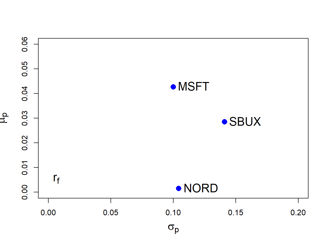
Figure 12.1: Risk-return characteristics of example data.
Clearly, Microsoft provides the best risk-return trade-off (i.e., has the highest Sharpe ratio) and Nordstorm provides with worst.
\(\blacksquare\)
Consider an equally weighted portfolio with \(x_{MSFT}=x_{NORD}=x_{SBUX}=1/3\). This portfolio has return \(R_{p,x}=\mathbf{x}^{\prime}\mathbf{R}\) where \(\mathbf{x}=(1/3,1/3,1/3)^{\prime}\). Using R, the portfolio mean and variance are:
## [1] 1mu.p.x = crossprod(x.vec,mu.vec)
sig2.p.x = t(x.vec)%*%sigma.mat%*%x.vec
sig.p.x = sqrt(sig2.p.x)
mu.p.x## [,1]
## [1,] 0.0242## [,1]
## [1,] 0.0759Next, consider another portfolio with weight vector \(\mathbf{y}=(y_{MSFT},y_{NORD},y_{SBUX})^{\prime}=(0.8,0.4,-0.2)^{\prime}\) and return \(R_{p,y}=\mathbf{y}^{\prime}\mathbf{R}\). The mean and volatility of this portfolio are:
y.vec = c(0.8, 0.4, -0.2)
names(y.vec) = asset.names
mu.p.y = crossprod(y.vec,mu.vec)
sig2.p.y = t(y.vec)%*%sigma.mat%*%y.vec
sig.p.y = sqrt(sig2.p.y)
mu.p.y
## [,1]
## [1,] 0.0291## [,1]
## [1,] 0.0966The covariance and correlation between \(R_{p,x}\) and \(R_{p,y}\) are:
##         [,1]
## [1,] 0.00391## [,1]
## [1,] 0.533The return and risk characteristics of the three assets together with portfolios x and y are illustrated in Figure 12.2. Notice that the equally weighted portfolio, portfolio x, has the smallest volatility.
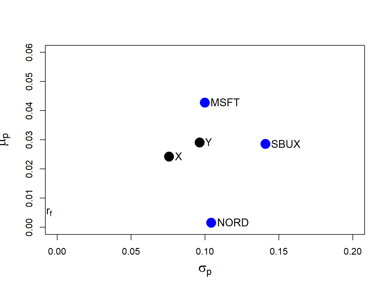
Figure 12.2: Risk-return characteristics of example data and portfolios with weight vectors \(\mathbf{x}=(0.333,0.333,0.333)^{\prime}\) and \(\mathbf{y}=(0.8,0.4,-0.2)^{\prime}\).
\(\blacksquare\)
Figure 12.2 shows that the risk-return points associated with portfolios of three assets do not fall nicely on a bullet-shaped line, as they do with two asset portfolios. In fact, the set of risk-return points generated by varying the three portfolio weights is a solid area. To see this, consider creating a set of 200 randomly generated three-asset portfolios whose weights sum to one:
set.seed(123)
x.msft = runif(200, min=-1.5, max=1.5)
x.nord = runif(200, min=-1.5, max=1.5)
x.sbux = 1 - x.msft - x.nord
head(cbind(x.msft, x.nord, x.sbux))
## x.msft x.nord x.sbux
## [1,] -0.637 -0.7838 2.4211
## [2,] 0.865 1.3871 -1.2520
## [3,] -0.273 0.3041 0.9690
## [4,] 1.149 0.0451 -0.1941
## [5,] 1.321 -0.2923 -0.0291
## [6,] -1.363 1.1407 1.2226Figure 12.3 shows the means and volatilities, as grey dots, of these 200 random portfolios of the three assets. Notice that the grey dots outline a bullet-shaped area (Markowitz bullet) that has an outer boundary that looks like the line characterizing the two-asset portfolio frontier. If we let the number of random portfolios get very large then the grey dots will fill in a solid area. At the tip of the Markowitz bullet is the minimum variance portfolio.
Recall the definition of a mean-variance efficient portfolio given in Chapter 11. For a fixed volatility \(\sigma_{p,0}\) the efficient portfolio is the one with the highest expected return. From Figure 12.3, we can see that efficient portfolios will lie on the outer boundary (above the minimum variance portfolio at the tip of the Markowitz bullet) of the set of feasible portfolios.
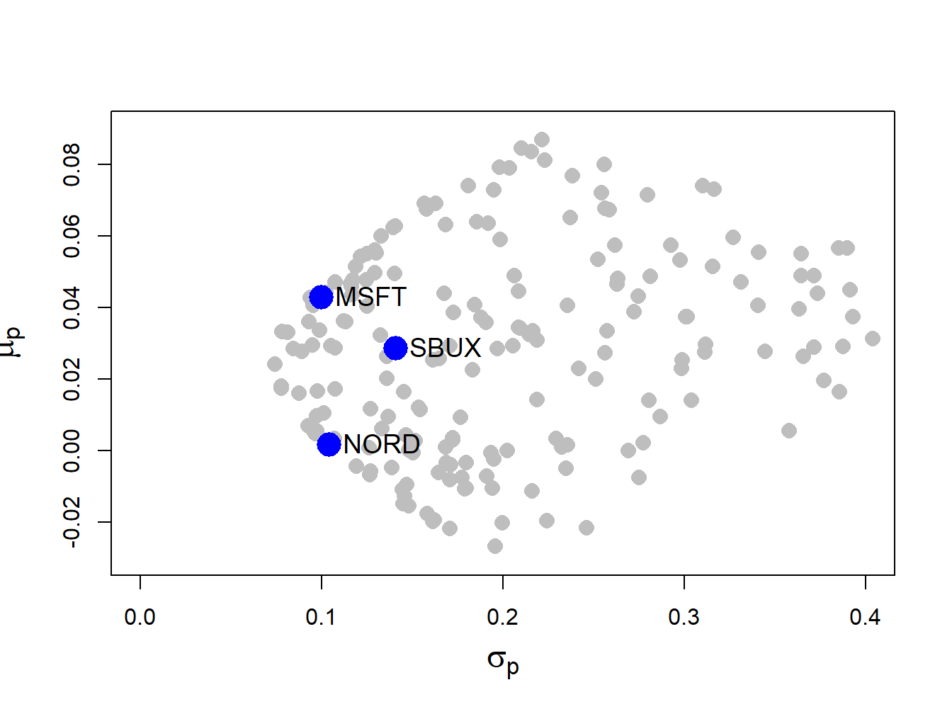
Figure 12.3: Risk-return characteristics of 200 random portfolios of three assets.
\(\blacksquare\)
12.1.2 Large portfolios and diversification
One of the key benefits of forming large portfolios is risk reduction due to portfolio diversification. Generally, a diversified portfolio is one in which wealth is spread across many assets.
To illustrate the impact of diversification on the risk of large portfolios, consider an equally weighted portfolio of \(N\) risky assets where \(N\) is a large number (e.g., \(N>100)\). Here, \(x_{i}=1/N\) and the \(N\times1\) portfolio weight vector is \(\mathbf{x}=(1/N,1/N,\ldots,1/N)^{\prime}=(1/N)(1,1,\ldots,1)^{\prime}=(1/N)\mathbf{1}\) where \(\mathbf{1}\) is an \(N\times1\) vector of ones. Let the \(N\times1\) return vector \(\mathbf{R}\) be described by the GWN model so that \(\mathbf{R}\sim N(\mu,\Sigma)\). The portfolio return is \(R_{p,x}=\mathbf{x}^{\prime}\mathbf{R}=(1/N)\mathbf{1}^{\prime}\mathbf{R}=(1/N)\sum_{i=1}^{N}R_{i}.\) The variance of this portfolio is: \[ \mathrm{var}(R_{p,x})=\mathrm{var}(\mathbf{x}^{\prime}\mathbf{R})=\mathrm{var}\left(\frac{1}{N}\mathbf{1}^{\prime}\mathbf{R}\right)=\frac{1}{N^{2}}\mathbf{1}^{\prime}\Sigma\mathbf{1}. \] Now, \[\begin{align*} \mathbf{1}^{\prime}\Sigma\mathbf{1}&=(\begin{array}{cccc} 1 & 1 & \ldots & 1\end{array})^{\prime}\left(\begin{array}{cccc} \sigma_{1}^{2} & \sigma_{12} & \ldots & \sigma_{1N}\\ \sigma_{12} & \sigma_{2}^{2} & \ldots & \sigma_{2N}\\ \vdots & \vdots & \ddots & \vdots\\ \sigma_{1N} & \sigma_{2N} & \ldots & \sigma_{N}^{2} \end{array}\right)\left(\begin{array}{c} 1\\ 1\\ \vdots\\ 1 \end{array}\right)\\ &=\text{ sum of all elements in } \Sigma. \end{align*}\] As a result, we can write: \[ \mathbf{1}^{\prime}\Sigma\mathbf{1}=\sum_{i=1}^{N}\sigma_{i}^{2}+\sum_{j\neq i}\sigma_{ij}, \] which is the sum of the \(N\) diagonal variance terms plus the \(N(N-1)\) off-diagonal covariance terms. Define the average variance as the average of the diagonal terms of \(\Sigma\): \[ \overline{\mathrm{var}}=\frac{1}{N}\sum_{i=1}^{N}\sigma_{i}^{2}, \] and the average covariance as the average of the off-diagonal terms of \(\Sigma\): \[ \overline{\mathrm{cov}}=\frac{1}{N(N-1)}\sum_{j\neq i}\sigma_{ij}. \] Then \(\mathbf{1}^{\prime}\Sigma\mathbf{1}=N\overline{\mathrm{var}}+N(N-1)\overline{\mathrm{cov}}\) and \(\mathrm{var}(R_{p,x})\) reduces to: \[\begin{eqnarray} \mathrm{var}(R_{p,x}) & = & \frac{1}{N^{2}}\mathbf{1}^{\prime}\Sigma\mathbf{1}=\frac{1}{N}\overline{\mathrm{var}}+\frac{N(N-1)}{N^{2}}\overline{\mathrm{cov}}\nonumber \\ & = & \frac{1}{N}\overline{\mathrm{var}}+\left(1-\frac{1}{N}\right)\overline{\mathrm{cov}}.\tag{12.1} \end{eqnarray}\] If \(N\) is reasonably large (e.g. \(N>100\)) then \[ \frac{1}{N}\overline{\mathrm{var}}\approx0\,\mathrm{and}\,\frac{1}{N}\overline{\mathrm{cov}}\approx0, \] so that \[ \mathrm{var}(R_{p,x})\approx\overline{\mathrm{cov}}. \] Hence, in a large diversified portfolio the portfolio variance is approximately equal to the average of the pairwise covariances. So what matters for portfolio risk is not the individual asset variances but rather the average of the asset covariances. In particular, portfolios with highly positively correlated returns will have higher portfolio variance than portfolios with less correlated returns.
Equation (12.1) also shows that portfolio variance should be a decreasing function of the number of assets in the portfolio, and that this function should level off at \(\overline{\mathrm{cov}}\) for large \(N\).