8.5 The Jackknife

Let $\theta$ denote a scalar parameter of interest. It could be a scalar parameter of the GWN model (e.g. $\mu$ or $\sigma$) or it could be a scalar function of the parameters of the GWN model (e.g. VaR or SR). Let $\hat{\theta}$ denote the plug-in estimator of $\theta$. The goal is to compute a numerical estimated standard error for $\hat{\theta}$, $\widehat{\mathrm{se}}(\hat{\theta})$, using the jackknife resampling method.

The jackknife resampling method utilizes $T$ resamples of the original data $\left\{ R_t \right\}_{t=1}^{T}$. The resamples are created by leaving out a single observation. For example, the first jackknife resample leaves out the first observation and is given by $\left\{ R_t \right\}_{t=2}^{T}$. This sample has $T-1$ observations. In general, the $t^{th}$ jackknife resample leaves out the $t^{th}$ return $R_{t}$ for $t \le T$. Now, on each of the $t=1,\ldots, T$ jackknife resamples you compute an estimate of $\theta$. Denote this jackknife estimate $\hat{\theta}_{-t}$ to indicate that $\theta$ is estimated using the resample that omits observation $t$. The estimator $\hat{\theta}_{-t}$ is called the leave-one-out estimator of $\theta$. Computing $\hat{\theta}_{-t}$ for $t=1,\ldots, T$ gives $T$ leave-one-out estimators $\left\{ \hat{\theta}_{-t} \right\}_{t=1}^{T}$.

The jackknife estimator of $\widehat{\mathrm{se}}(\hat{\theta})$ is the scaled standard deviation of $\left\{ \hat{\theta}_{-t} \right\}_{t=1}^{T}$:

$$\begin{equation} \widehat{\mathrm{se}}_{jack}(\hat{\theta}) = \sqrt{ \frac{T-1}{T}\sum_{t=1}^T (\hat{\theta}_{-t} - \bar{\theta})^2 }, \tag{8.10} \end{equation}$$

where $\bar{\theta} = T^{-1}\sum_{t=1}^T \hat{\theta}_{-t}$ is the sample mean of $\left\{ \hat{\theta}_{-t} \right\}_{t=1}^{T}$. The estimator (8.10) is easy to compute and does not require any analytic calculations from the asymptotic distribution of $\hat{\theta}$.

The intuition for the jackknife standard error formula can be illustrated by considering the jackknife standard error estimate for the sample mean $\hat{\theta} = \hat{\mu}$. We know that the analytic estimated squared standard error for $\hat{\mu}$ is

$$\begin{equation*} \widehat{\mathrm{se}}(\hat{\mu})^2 = \frac{\hat{\sigma}^2}{T} = \frac{1}{T} \frac{1}{T-1} \sum_{t=1}^T (R_t - \hat{\mu})^2. \end{equation*}$$

Now consider the jackknife squared standard error for $\hat{\mu}$:

$$\begin{equation*} \widehat{\mathrm{se}}_{jack}(\hat{\mu})^2= \frac{T-1}{T}\sum_{t=1}^T (\hat{\mu}_{-t} - \bar{\mu})^2, \end{equation*}$$

where $\bar{\mu} = T^{-1}\sum_{t=1}^T \hat{\mu}_{-t}$. Here, we will show that $\widehat{\mathrm{se}}(\hat{\mu})^2 = \widehat{\mathrm{se}}_{jack}(\hat{\mu})^2$.

First, note that

$$\begin{align*} \hat{\mu}_{-t} & = \frac{1}{T-1}\sum_{j \ne t} R_j = \frac{1}{T-1} \left( \sum_{j=1}^T R_j - R_t \right) \\ &= \frac{1}{T-1} \left( T \hat{\mu} - R_t \right) \\ &= \frac{T}{T-1}\hat{\mu} - \frac{1}{T-1}R_t. \end{align*}$$

Next, plugging in the above to the definition of $\bar{\mu}$ we get

$$\begin{align*} \bar{\mu} &= \frac{1}{T} \sum_{j=1}^T \hat{\mu}_{-t} = \frac{1}{T}\sum_{t=1}^T \left( \frac{T}{T-1}\hat{\mu} - \frac{1}{T-1}R_t \right) \\ &= \frac{1}{T-1} \sum_{t=1}^T \hat{\mu} - \frac{1}{T}\frac{1}{T-1} \sum_{t=1}^T R_t \\ &= \frac{T}{T-1} \hat{\mu} - \frac{1}{T-1} \hat{\mu} \\ &= \hat{\mu} \left( \frac{T}{T-1} - \frac{1}{T-1} \right) \\ &= \hat{\mu}. \end{align*}$$

Hence, the sample mean of $\hat{\mu}_{-t}$ is $\hat{\mu}$. Then we can write

$$\begin{align*} \hat{\mu}_{-t} - \bar{\mu} & = \hat{\mu}_{-t} - \hat{\mu} \\ & = \frac{T}{T-1}\hat{\mu} - \frac{1}{T-1}R_t - \hat{\mu} \\ &= \frac{T}{T-1}\hat{\mu} - \frac{1}{T-1}R_t - \frac{T-1}{T-1}\hat{\mu} \\ &= \frac{1}{T-1}\hat{\mu} - \frac{1}{T-1}R_t \\ &= \frac{1}{T-1}(\hat{\mu} - R_t). \end{align*}$$

Using the above we can write

$$\begin{align*} \widehat{\mathrm{se}}_{jack}(\hat{\mu})^2 &= \frac{T-1}{T}\sum_{t=1}^T (\hat{\mu}_{-t} - \bar{\mu})^2 \\ &= \frac{T-1}{T}\left(\frac{1}{T-1}\right)^2 \sum_{t=1}^T (\hat{\mu} - R_t)^2 \\ &= \frac{1}{T}\frac{1}{T-1} \sum_{t=1}^T (\hat{\mu} - R_t)^2 \\ &= \frac{1}{T} \hat{\sigma}^2 \\ &= \widehat{\mathrm{se}}(\hat{\mu})^2. \end{align*}$$

Example 2.22 (Jackknife standard error for $\hat{\mu}$ for Microsoft)

We can compute the leave-one-out estimates $\{\hat{\mu}_{-t}\}_{t=1}^T$ using a simple for loop as follows:

n.obs = length(msftRetS)
muhat.loo = rep(0, n.obs)
for(i in 1:n.obs) {
  muhat.loo[i] = mean(msftRetS[-i])
}

In the above loop, msftRetS[-i] extracts all observations except observation $i$. The mean of the leave-one-out estimates is

mean(muhat.loo)

## [1] 0.00915

which is the sample mean of msftRetS. It is informative to plot a histogram of the leave-one-out estimates:

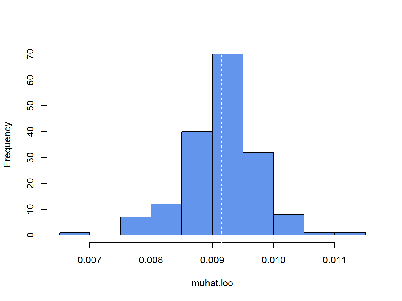
Figure 8.1: Histogram of leave-one-out estimator of $\mu$ for Microsoft.

The white dotted line is at the point $\hat{\mu} = 0.00915$. The jackknife estimated standard error is the scaled standard deviation of the $T$ $\hat{\mu}_{-t}$ values:⁴¹

se.jack.muhat = sqrt(((n.obs - 1)^2)/n.obs)*sd(muhat.loo)
se.jack.muhat

## [1] 0.00774

This value is exactly the same as the analytic standard error:

se.muhatS

## [1] 0.00774

You can also compute jackknife estimated standard errors using the bootstrap function jackknife:

library(bootstrap)
muhat.jack = jackknife(coredata(msftRetS), mean)
names(muhat.jack)

## [1] "jack.se"     "jack.bias"   "jack.values" "call"

By default, jackknife() takes as input a vector of data and the name of an R function and returns a list with components related to the jackknife procedure. The component jack.values contains the leave-one-out estimators, and the component jack.se gives you the jackknife estimated standard error:

muhat.jack$jack.se

## [1] 0.00774

$\blacksquare$

The fact that the jackknife standard error estimate for $\hat{\mu}$ equals the analytic standard error is main justification for using the jackknife to compute standard errors. For estimated parameters other than $\hat{\mu}$ and general estimated functions the jackknife standard errors are often numerically very close to the delta method standard errors. The following example illustrates this point for the example functions (8.1) - (8.4).

Example 2.25 (Jackknife standard errors for plug-in estimators of example functions)

Here, we use the bootstrap function jackknife() to compute jackknife estimated standard errors for the plug-in estimates of the example functions (8.1) - (8.4) and we compare the jackknife standard errors with the delta method standard errors. To use jackknife() with user-defined functions involving multiple parameters you must create the function such that the first input is an integer vector of index observations and the second input is the data. For example, a function for computing (8.1) to be passed to jackknife() is:

theta.f1 = function(x, xdata) {
  mu.hat = mean(xdata[x, ])
  sigma.hat = sd(xdata[x, ])
  fun.hat = mu.hat + sigma.hat*qnorm(0.05)
  fun.hat
}

To compute the jackknife estimated standard errors for the estimate of (8.1) use:

f1.jack = jackknife(1:n.obs, theta=theta.f1, coredata(msftRetS))
ans = cbind(f1.jack$jack.se, dm1$SE)
colnames(ans) = c("Jackknife", "Delta Method")
rownames(ans) = "f1"
ans

##    Jackknife Delta Method
## f1    0.0133       0.0119

Here, we see that the estimated jackknife standard error for $f_1(\hat{\theta})$ is very close to the delta method standard error computed earlier.

To compute the jackknife estimated standard error for $f_2(\hat{\theta})$ use:

theta.f2 = function(x, xdata, W0) {
  mu.hat = mean(xdata[x, ])
  sigma.hat = sd(xdata[x, ])
  fun.hat = -W0*(mu.hat + sigma.hat*qnorm(0.05))
  fun.hat
}
f2.jack = jackknife(1:n.obs, theta=theta.f2, coredata(msftRetS), W0)
ans = cbind(f2.jack$jack.se, dm2$SE)
colnames(ans) = c("Jackknife", "Delta Method")
rownames(ans) = "f2"
ans

##    Jackknife Delta Method
## f2      1329         1187

Again, the jackknife standard error is close to the delta method standard error.

To compute the jackknife estimated standard error for $f_3(\hat{\theta})$ use:

theta.f3 = function(x, xdata, W0) {
  mu.hat = mean(xdata[x, ])
  sigma.hat = sd(xdata[x, ])
  fun.hat = -W0*(exp(mu.hat + sigma.hat*qnorm(0.05)) - 1)
  fun.hat
}
f3.jack = jackknife(1:n.obs, theta=theta.f3, coredata(msftRetC), W0)
ans = cbind(f3.jack$jack.se, dm3$SE)
colnames(ans) = c("Jackknife", "Delta Method")
rownames(ans) = "f3"
ans

##    Jackknife Delta Method
## f3      1315          998

For log-normal VaR, the jackknife standard error is a bit larger than the delta method standard error.

Finally, to compute the jacknife estimated standard for the Sharpe ratio use:

theta.f4 = function(x, xdata, r.f) {
  mu.hat = mean(xdata[x, ])
  sigma.hat = sd(xdata[x, ])
  fun.hat = (mu.hat-r.f)/sigma.hat
  fun.hat
}
f4.jack = jackknife(1:n.obs, theta=theta.f4, coredata(msftRetS), r.f)
ans = cbind(f4.jack$jack.se, dm4$SE)
colnames(ans) = c("Jackknife", "Delta Method")
rownames(ans) = "f4"
ans

##    Jackknife Delta Method
## f4     0.076       0.0763

Here, the jackknife and delta method standard errors are very close.

$\blacksquare$

8.5.1 The jackknife for vector-valued estimates

The jackknife can also be used to compute an estimated variance matrix of a vector-valued estimate of parameters. Let $\theta$ denote a $k \times 1$ vector of GWN model parameters (e.g. $\theta=(\mu,\sigma)'$), and let $\hat{\theta}$ denote the plug-in estimate of $\theta$. Let $\hat{\theta}_{-t}$ denote the leave-one-out estimate of $\theta$, and $\bar{\theta}=T^{-1}\sum_{t=1}^T \hat{\theta}_{-t}$. Then the jackknife estimate of the $k \times k$ variance matrix $\widehat{\mathrm{var}}(\hat{\theta})$ is the scaled sample covariance of $\{\hat{\theta}_{-t}\}_{t=1}^T$:

$$\begin{equation} \widehat{\mathrm{var}}_{jack}(\hat{\theta}) = \frac{T-1}{T} \sum_{t=1}^T (\hat{\theta}_{-t} - \bar{\theta})(\hat{\theta}_{-t} - \bar{\theta})'. \tag{8.11} \end{equation}$$

The jackknife estimated standard errors for the elements of $\hat{\theta}$ are given by the square root of the diagonal elements of $\widehat{\mathrm{var}}_{jack}(\hat{\theta})$.

The same principle works for computing the estimated variance matrix of a vector of functions of GWN model parameters. Let $f:R^k \rightarrow R^l$ with $l \le k$ and define $\eta = f(\theta)$ denote a $l \times 1$ vector of functions of GWN model parameters. Let $\hat{\eta}=f(\hat{\theta})$ denote the plug-in estimator of $\eta$. Let $\hat{\eta}_{-t}$ denote the leave-one-out estimate of $\eta$, and $\bar{\eta}=T^{-1}\sum_{t=1}^T \hat{\eta}_{-t}$. Then the jackknife estimate of the $l \times l$ variance matrix $\widehat{\mathrm{var}}(\hat{\eta})$ is the scaled sample covariance of $\{\hat{\eta}_{-t}\}_{t=1}^T$:

$$\begin{equation} \widehat{\mathrm{var}}_{jack}(\hat{\eta}) = \frac{T-1}{T} \sum_{t=1}^T (\hat{\eta}_{-t} - \bar{\eta})(\hat{\eta}_{-t} - \bar{\eta})'. \tag{8.12} \end{equation}$$

Example 3.8 (Jackknife variance estimate for $\hat{\theta} = (\mu,\sigma)'$ for Microsoft simple returns)

The bootstrap function jackknife() function only works for scalar-valued parameter estimates, so we have to compute the jackknife variance estimate by hand using a for loop. The R code is:

n.obs = length(msftRetS)
muhat.loo = rep(0, n.obs)
sigmahat.loo = rep(0, n.obs)
for(i in 1:n.obs) {
  muhat.loo[i] = mean(msftRetS[-i])
  sigmahat.loo[i] = sd(msftRetS[-i])
}
thetahat.loo = cbind(muhat.loo, sigmahat.loo)
colnames(thetahat.loo) = c("mu", "sigma")
varhat.jack = (((n.obs-1)^2)/n.obs)*var(thetahat.loo)
varhat.jack

##             mu    sigma
## mu    5.99e-05 1.49e-05
## sigma 1.49e-05 6.12e-05

The jackknife variance estimate is somewhat close to the analytic estimate:

var.thetahatS

##             mu    sigma
## mu    5.99e-05 0.00e+00
## sigma 0.00e+00 2.99e-05

Since the first element of $\hat{\theta}$ is $\hat{\mu}$, the (1,1) elements of the two variance matrix estimates match exactly. However, the varhat.jack has non-zero off diagonal elements and the (2,2) element corresponding to $\hat{\sigma}$ is considerably bigger than (2,2) element of the analytic estimate. Converting var.thetahatS to an estimated correlation matrix gives:

cov2cor(varhat.jack)

##          mu sigma
## mu    1.000 0.246
## sigma 0.246 1.000

Here, we see that the jackknife shows a small positive correlation between $\hat{\mu}$ and $\hat{\sigma}$ whereas the analytic matrix shows a zero correlation.

$\blacksquare$

8.5.2 Pros and Cons of the Jackknife

The jackknife gets its name because it is a useful statistical device.⁴² The main advantages (pros) of the jacknife are:

• It is a good “quick and dirty” method for computing numerical estimated standard errors of estimates that does not rely on asymptotic approximations.

• The jackknife estimated standard errors are often close to the delta method standard errors.

This jackknife, however, has some limitations (cons). The main limitations are:

• It can be computationally burdensome for very large samples (e.g., if used with ultra high frequency data).

• It does not work well for non-smooth functions such as empirical quantiles.

• It is not well suited for computing confidence intervals.

• It is not as accurate as the bootstrap.

---

41. the scaling of the standard deviation of $\hat{\mu}_{-t}$ is approximately $\sqrt{T}$.↩︎

42. A jackknife is also the name of a very useful folding knife.↩︎