5.4 Rolling descriptive statistics
The assumption that asset returns are covariance stationary implies that the asset return means (\(\mu_i\)), variances (\(\sigma_i^2\)), covariances (\(\sigma_{ij}\)), and correlations (\(\rho_{ij}\)) are constant over time for all assets \(i\) and \(j\). Essentially, this means that the economic environment remains constant over time. Clearly, this is a strong assumption and we have seen evidence in the graphical descriptive statistics that this assumption might be suspect. For example, we have seen that the volatility of asset returns appears to change over time. In this section, we introduce rolling descriptive statistics to further investigate the appropriateness of the covariance stationary assumption of asset returns.
A commonly used technique to investigate whether certain asset return characteristics are constant over time is to compute sample descriptive statistics over rolling sub-sample windows of fixed length. To illustrate, suppose one is interested in determining if the expected return parameter of an asset return \(\mu\) is constant over time. Assume returns are observed over a sample of size \(T\). An informal way to do this is to compute estimates of \(\mu\) over rolling windows of length \(n<T\):
\[\begin{align*} \hat{\mu}_{t}(n) & =\frac{1}{n}\sum_{k=0}^{n-1}r_{t-k}=\frac{1}{n}(r_{t}+r_{t-1}+\cdots+r_{t-n+1}), \end{align*}\]
for \(t=n,\ldots,T\). Here \(\hat{\mu}_{n}(n)\) is the sample mean of the returns \(\{r_{t}\}_{t=1}^{n}\) over the first sub-sample window of size \(n\). Then \(\hat{\mu}_{n+1}(n)\) is the sample mean of the returns \(\{r_{t}\}_{t=2}^{n+1}\) over the second sub-sample window of size \(n\). Continuing in this fashion we roll the sample window forward one observation at a time and compute \(\hat{\mu}_{t}(n)\) until we arrive at the last sub-sample window of size \(n\). The end result is \(T-n+1\) rolling estimates \(\left\{\hat{\mu}_{n}(n),\,\hat{\mu}_{n+1}(n),\ldots,\hat{\mu}_{T}(n)\right\}\).
If returns are covariance stationary then \(\mu\) is constant over time and we would expect that \(\hat{\mu}_{n}(n)\approx\hat{\mu}_{n+1}(n)\approx\cdots\approx\hat{\mu}_{T}(n)\). That is, the estimates of \(\mu\) over each rolling window should be similar. We would not expect them to be exactly equal due to sampling uncertainty but they should not be drastically different. In contrast, if returns are not covariance stationary due to time variation in \(\mu\) then we would expect to see meaningful time variation in the rolling estimates \(\left\{\hat{\mu}_{n}(n),\,\hat{\mu}_{n+1}(n),\ldots,\hat{\mu}_{T}(n)\right\}\).
A natural way to see the time variation in \(\{\hat{\mu}_{t}(n)\}_{t=n}^T\) is to make a time series plot of these rolling estimates as illustrated in the next example.
Consider computing rolling estimates of \(\mu\) for Microsoft, Starbucks
and the S&P 500 index returns. You can easily do this using the zoo
function rollapply(), which applies a user-specified function
to a time series over rolling windows of fixed size. The arguments
to rollapply() are:
## function (data, width, FUN, ..., by = 1, by.column = TRUE, fill = if (na.pad) NA,
##     na.pad = FALSE, partial = FALSE, align = c("center", "left",
##         "right"), coredata = TRUE)
## NULL
where data is either a "zoo" or "xts" object, width is the window width, FUN is the R
function to be applied over the rolling windows, ... are any optional arguments to be supplied to FUN, by
specifies how many observations to increment the rolling windows, by.column specifies if FUN is to be applied to each
column of data or to be applied to all columns of data, and align specifies the location of the time index in the window. The function returns an “xts/zoo” object containing the rolling estimates.
For example, to compute 24-month rolling estimates of \(\mu\) for Microsoft, S&P 500 index, and simulated GWN data (that matches the mean and volatility of Microsoft returns), incremented by one month with the time index aligned to the end of the window use:
roll.data = merge(msftMonthlyRetS,sp500MonthlyRetS,gwnMonthly)
colnames(roll.data) = c("MSFT", "SP500", "GWN")
roll.muhat = rollapply(roll.data, width=24, by=1, by.column=TRUE,
                       FUN=mean, align="right")
class(roll.muhat)
## [1] "xts" "zoo"The object roll.muhat is an “xts” object with three columns giving the rolling mean estimates for the GWN data, Microsoft, and the S&P 500 index. The first 23 months of data are NA as we need at least 24 months of data to compute the first rolling estimates:
##          MSFT SP500 GWN
## Feb 1998   NA    NA  NA
## Mar 1998   NA    NA  NA
## Apr 1998   NA    NA  NA
The first rolling estimates are for the 24-months just prior to January, 2000 and the last rolling estimates are for the 24-months just prior to May 2012.
##            MSFT  SP500       GWN
## Jan 2000 0.0487 0.0161 -1.68e-03
## Feb 2000 0.0394 0.0124 -9.85e-05
## Mar 2000 0.0450 0.0143 1.39e-02## MSFT SP500 GWN
## Mar 2012 0.00869 0.00894 -0.0307
## Apr 2012 0.00661 0.00801 -0.0324
## May 2012 0.00948 0.00882 -0.0298The rolling means are shown in Figure 5.29 created using:
plot(roll.muhat, main="", multi.panel=FALSE, lwd=2,
     col=c("black", "red", "green"), lty=c("solid", "solid", "solid"),
     major.ticks="years", grid.ticks.on="years",
     legend.loc = "topright")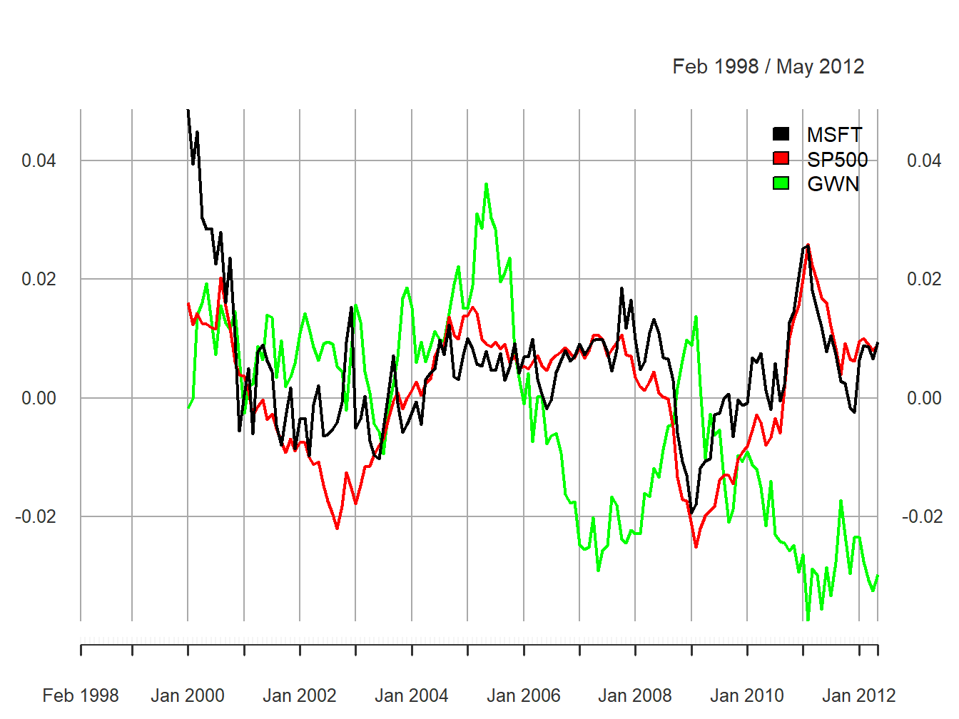
Figure 5.29: 24-month rolling estimates of \(\mu\)
All of the rolling estimates show time variation over the sample, including the simulated GWN returns which have a constant mean by construction. The ranges of the rolling estimates are:
##        MSFT   SP500     GWN
## Min -0.0194 -0.0251 -0.0376
## Max  0.0487  0.0260  0.0362
Interestingly, the rolling estimates for Microsoft and the S&P 500 index exhibit a similar pattern of time variation. The estimates start positive at the end of the dot-com boom, decrease from 2000 to mid 2002 (Microsoft and the S&P 500 index become negative), increase from 2003 to 2006 during the booming economy, fall sharply during the financial crisis period 2007 to 2009, and increase from 2009 to 2011, and decrease afterward. The Microsoft and S&P 500 estimates follow each other very closely due to their moderately strong positive correlation of 0.614. Somewhat surprisingly, the rolling means for the simulated GWN data also show substantial time variation over the sample. Since the true mean of the simulated GWN data is constant, the variation observed in the rolling means represents sampling uncertainty due to the small sample sizes of the rolling means. The magnitude of the variation in the rolling mean estimates for the GWN data should make us pause in concluding there is substantial change in the mean estimates of Microsoft (and possibly the S&P 500). However, the fact that the rolling estimates for Microsoft and the S&P 500 index behave as expected during the booms and busts strongly suggests that the underlying mean values for these assets are not constant over the full sample.
\(\blacksquare\)
To investigate time variation in return volatility, we can compute rolling estimates of \(\sigma^{2}\) and \(\sigma\) over fixed windows of size \(n<T\): \[\begin{align*} \hat{\sigma}_{t}^{2}(n) & =\frac{1}{n-1}\sum_{k=0}^{n-1}(r_{t-k}-\hat{\mu}_{t}(n))^{2},\\ \hat{\sigma}_{t}(n) & =\sqrt{\hat{\sigma}_{t}^{2}(n)}. \end{align*}\] If return volatility is constant over time, then we would expect that \(\hat{\sigma}_{n}(n)\approx\hat{\sigma}_{n+1}(n)\approx\cdots\approx\hat{\sigma}_{T}(n)\). That is, the estimates of \(\sigma\) over each rolling window should be similar. In contrast, if volatility is not constant over time then we would expect to see meaningful time variation in the rolling estimates \(\left\{\hat{\sigma}_{n}(n),\,\hat{\sigma}_{n+1}(n),\ldots,\hat{\sigma}_{T}(n)\right\}\).
To compute and plot 24-month rolling estimates of \(\sigma\) for Microsoft, S&P 500 index, and GWN returns incremented by one month with the time index aligned to the beginning of the window use:
The rolling estimates are illustrated in Figure 5.30.
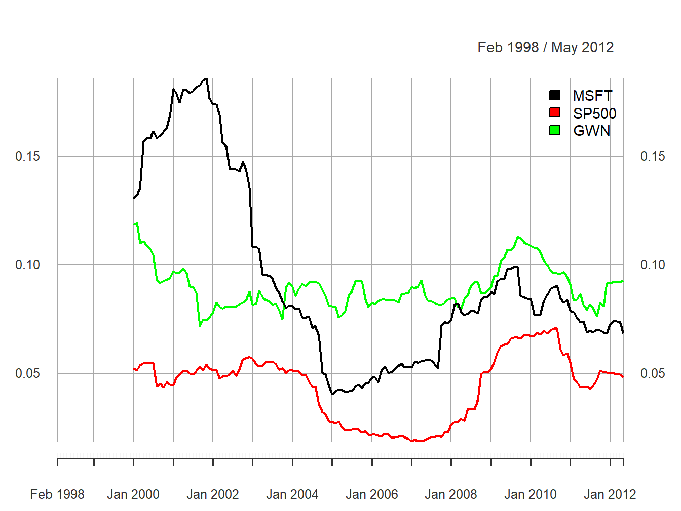
Figure 5.30: 24-month rolling estimates of \(\sigma\).
The rolling volatilities for Microsoft and the S&P 500 index show a similar pattern of time variation over the sample but the Microsoft volatilities are considerably more variable:
##       MSFT  SP500    GWN
## Min 0.0402 0.0186 0.0716
## Max 0.1863 0.0706 0.1192
The rolling volatilities for Microsoft peak at about \(18\%\) per month at the end of the dot-com boom, fall sharply to about \(4\%\) per month at the beginning of 2005, then level off until the beginning of the financial crisis, and increase during the financial crisis to about \(10\%\) per month and fall slightly afterward. The S&P 500 volatilities have a similar pattern as the Microsoft volatilities but their movements are not as extreme. In contrast, the rolling volatilities of the GWN series are fairly stable bouncing between \(7\%\) and \(12\%\). The time variation exhibited by the rolling volatilities of Microsoft and the S&P 500 index places additional doubt on the covariance stationarity assumption for returns.
\(\blacksquare\)
To investigate time variation in the correlation between two asset returns, \(\rho_{ij}\), one can compute the rolling covariances and correlations over fixed windows of size \(n<T\): \[\begin{align*} \hat{\sigma}_{ij,t}(n) & =\frac{1}{n-1}\sum_{k=0}^{n-1}(r_{i,t-k}-\hat{\mu}_{i}(n))(r_{j,t-k}-\hat{\mu}_{j}(n)),\\ \hat{\rho}_{ij,t}(n) & =\frac{\hat{\sigma}_{ij,t}(n)}{\hat{\sigma}_{i,t}(n)\hat{\sigma}_{j,t}(n)}. \end{align*}\]
A function to compute the pair-wise sample correlations between Microsoft, Starbucks and the S&P 500 index is
rhohat = function(x) {
   corhat = cor(x)
   corhat.vals = corhat[lower.tri(corhat)]
   names(corhat.vals) = c("MSFT.SP500", "MSFT.GWN", "SP500.GWN")
   corhat.vals
}
Using the function rhohat(), 24-month rolling estimates of
\(\rho_{ij}\) for Microsoft, Starbucks and the S&P 500 index incremented
by one month with the time index aligned to the beginning of the window
can be computed using
roll.rhohat = rollapply(roll.data, width=24, FUN=rhohat,
   by=1, by.column=FALSE, align="right")
head(na.omit(roll.rhohat),n=3)
## MSFT.SP500 MSFT.GWN SP500.GWN
## Jan 2000 0.638 0.392 0.278
## Feb 2000 0.637 0.345 0.244
## Mar 2000 0.663 0.415 0.377Notice that by.column=FALSE in the call to rollapply().
This is necessary as the function rhohat() operates on all
columns of the data object roll.data. The rolling estimates
are illustrated in Figure 5.31.
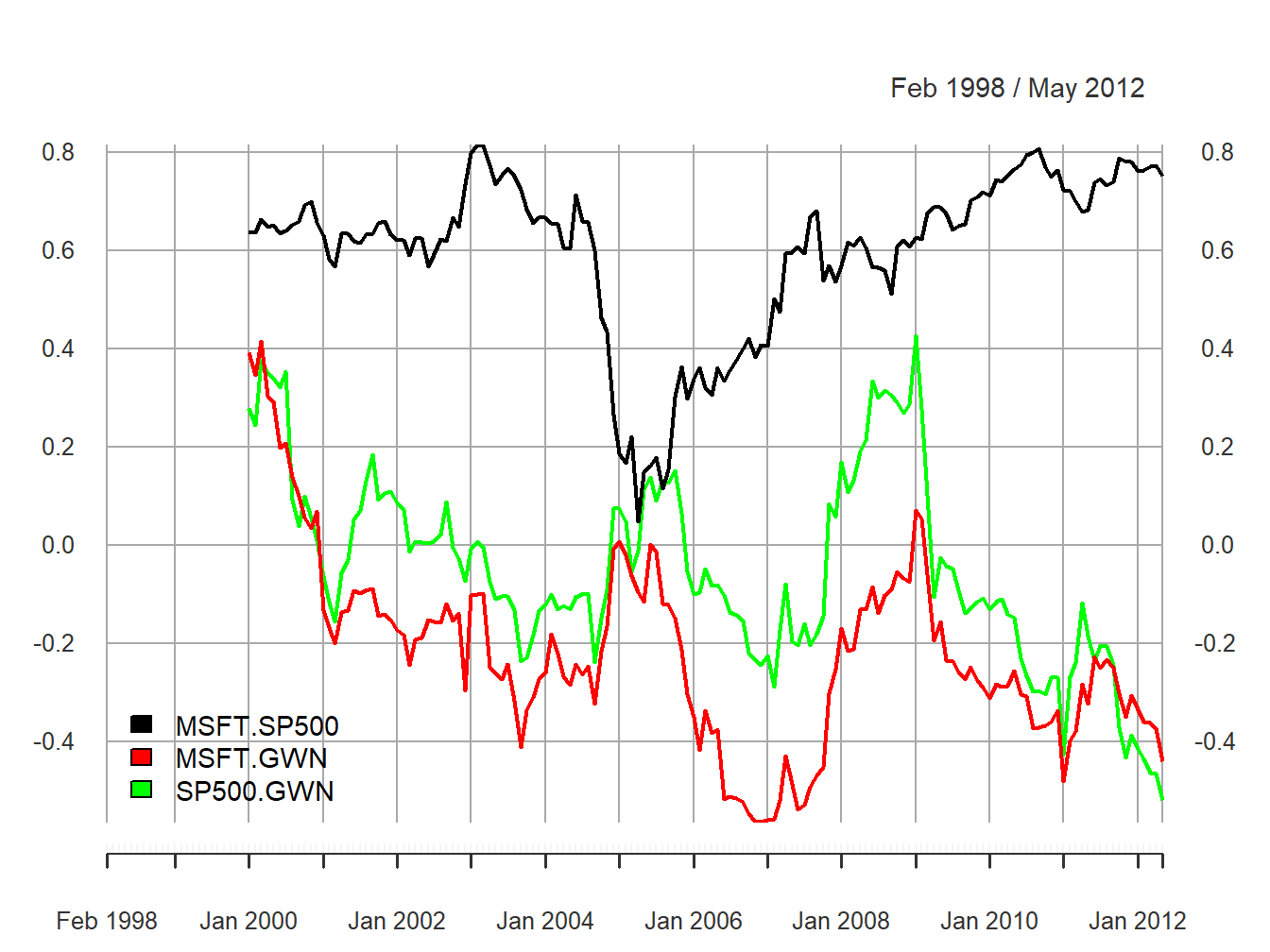
Figure 5.31: 24-month rolling estimates of \(\rho_{ij}\) for Microsoft, Starbucks and the S&P 500 index.
The ranges of the rolling correlations are:
##     MSFT.SP500 MSFT.GWN SP500.GWN
## Min     0.0487   -0.565    -0.521
## Max     0.8169    0.415     0.428
The rolling correlations between Microsoft and the S&P 500 index show an interesting pattern. They start moderately high, around 0.6, then plunge to about 0.05 in early 2005, and then gradually pick back up to about 0.8 at the end of the sample. The rolling correlations are highest during the financial crisis periods and lowest during the calm periods. Interestingly, the rolling correlations between the GWN series and Microsoft, and the GWN series and the S&P 500 index fluctuate somewhat randomly between -0.5 and 0.5 and show no particular pattern. There is compelling evidence that the correlation between Microsoft and the S&P 500 index is not constant over time.
\(\blacksquare\)
It must be kept in mind that the rolling descriptive statistics are informal diagnostics for evaluating the assumption of covariance stationarity. As we have seen, there is considerably sampling variability in the rolling statistics due to the small window size which can make it difficult to untangle statistical noise from true changes in the underlying parameters. In Chapter 9 we will consider formal statistical tests for constant parameters that can give better evidence for or against the assumption of covariance stationarity.
5.4.1 Practical issues associated with rolling estimates
To be completed
- Discuss choice of window width. Small window widths tend to produce choppy estimates with a lot of estimation error. Large window widths produce smooth estimates with less estimation error
- Discuss choice of increment. For a given window width, the roll-by increment determines the number of overlapping returns in each window. Number of overlapping returns is \(n-incr\) where \(n\) is the window width and \(incr\) is the roll-by increment. Incrementing the window by 1 gives the largest number of over lapping returns. If \(incr\geq n\) then the rolling windows are non-overlapping.
- A large positive or negative return in a window can greatly influence the estimate and cause a drop-off effect as the window rolls past the large observation.