7.2 Finite Sample Properties of Estimators

Consider $\hat{\theta}$ as a random variable. In general, the pdf of $\hat{\theta}$, $f(\hat{\theta})$, depends on the pdf’s of the random variables $\{R_{t}\}_{t=1}^{T}$. The exact form of $f(\hat{\theta})$ may be very complicated. Sometimes we can use analytic calculations to determine the exact form of $f(\hat{\theta})$. This can be done, for example, when $\hat{\theta} = \hat{\mu}$. In general, the exact form of $f(\hat{\theta})$ is often too difficult to derive exactly. When $f(\hat{\theta})$ is too difficult to compute we can often approximate $f(\hat{\theta})$ using either Monte Carlo simulation techniques or the Central Limit Theorem (CLT). In Monte Carlo simulation, we use the computer to simulate many different realizations of the random returns $\{R_{t}\}_{t=1}^{T}$ and on each simulated sample we evaluate the estimator $\hat{\theta}$. The Monte Carlo approximation of $f(\hat{\theta})$ is the empirical distribution of $\hat{\theta}$ over the different simulated samples. For a given sample size $T$, Monte Carlo simulation gives a very accurate approximation to $f(\hat{\theta})$ if the number of simulated samples is very large. The CLT approximation of $f(\hat{\theta})$ is a normal distribution approximation that becomes more accurate as the sample size $T$ gets very large. An advantage of the CLT approximation is that it is often easy to compute. The disadvantage is that the accuracy of the approximation depends on the estimator $\hat{\theta}$ and sample size $T$.

For analysis purposes, we often focus on certain characteristics of $f(\hat{\theta})$, like its expected value (center), variance and standard deviation (spread about expected value)$.$ The expected value of an estimator is related to the concept of estimator bias, and the variance/standard deviation of an estimator is related to the concept of estimator precision. Different realizations of the random variables $\{R_{t}\}_{t=1}^{T}$ will produce different values of $\hat{\theta}$. Some values of $\hat{\theta}$ will be bigger than $\theta$ and some will be smaller. Intuitively, a good estimator of $\theta$ is one that is on average correct (unbiased) and never gets too far away from $\theta$ (small variance). That is, a good estimator will have small bias and high precision.

7.2.1 Bias

Bias concerns the location or center of $f(\hat{\theta})$ in relation to $\theta$. If $f(\hat{\theta})$ is centered away from $\theta$, then we say $\hat{\theta}$ is a biased estimator of $\theta$. If $f(\hat{\theta})$ is centered at $\theta$, then we say that $\hat{\theta}$ is an unbiased estimator of $\theta$. Formally, we have the following definitions:

Definition 4.1 The estimation error is the difference between the estimator and the parameter being estimated:

$$\begin{equation} \mathrm{error}(\hat{\theta},\theta)=\hat{\theta}-\theta.\tag{7.2} \end{equation}$$

Definition 2.4 The bias of an estimator $\hat{\theta}$ of $\theta$ is the expected estimation error: $$\begin{equation} \mathrm{bias}(\hat{\theta},\theta)=E[\mathrm{error}(\hat{\theta},\theta)]=E[\hat{\theta}]-\theta.\tag{7.3} \end{equation}$$

Definition 2.5 An estimator $\hat{\theta}$ of $\theta$ is unbiased if $\mathrm{bias}(\hat{\theta},\theta)=0$; i.e., if $E[\hat{\theta}]=\theta$ or $E[\mathrm{error}(\hat{\theta},\theta)]=0$.

Unbiasedness is a desirable property of an estimator. It means that the estimator produces the correct answer “on average”, where “on average” means over many hypothetical realizations of the random variables $\{R_{t}\}_{t=1}^{T}$. It is important to keep in mind that an unbiased estimator for $\theta$ may not be very close to $\theta$ for a particular sample, and that a biased estimator may actually be quite close to $\theta$. For example, consider two estimators of $\theta$, $\hat{\theta}_{1}$ and $\hat{\theta}_{2}$. The pdfs of $\hat{\theta}_{1}$ and $\hat{\theta}_{2}$ are illustrated in Figure 7.1. $\hat{\theta}_{1}$ is an unbiased estimator of $\theta$ with a large variance, and $\hat{\theta}_{2}$ is a biased estimator of $\theta$ with a small variance. Consider first, the pdf of $\hat{\theta}_{1}$. The center of the distribution is at the true value $\theta=0$, $E[\hat{\theta}_{1}]=0$, but the distribution is very widely spread out about $\theta=0$. That is, $\mathrm{var}(\hat{\theta}_{1})$ is large. On average (over many hypothetical samples) the value of $\hat{\theta}_{1}$ will be close to $\theta$, but in any given sample the value of $\hat{\theta}_{1}$ can be quite a bit above or below $\theta$. Hence, unbiasedness by itself does not guarantee a good estimator of $\theta$. Now consider the pdf for $\hat{\theta}_{2}$. The center of the pdf is slightly higher than $\theta=0$, i.e., $\mathrm{bias}(\hat{\theta}_{2},\theta)>0$, but the spread of the distribution is small. Although the value of $\hat{\theta}_{2}$ is not equal to 0 on average we might prefer the estimator $\hat{\theta}_{2}$ over $\hat{\theta}_{1}$ because it is generally closer to $\theta=0$ on average than $\hat{\theta}_{1}$.

While unbiasedness is a desirable property of an estimator $\hat{\theta}$ of $\theta$, it, by itself, is not enough to determine if $\hat{\theta}$ is a good estimator. Being correct on average means that $\hat{\theta}$ is seldom exactly correct for any given sample. In some samples $\hat{\theta}$ is less than $\theta$, and some samples $\hat{\theta}$ is greater than $\theta$. More importantly, we need to know how far $\hat{\theta}$ typically is from $\theta$. That is, we need to know about the magnitude of the spread of the distribution of $\hat{\theta}$ about its average value. This will tell us the precision of $\hat{\theta}$.

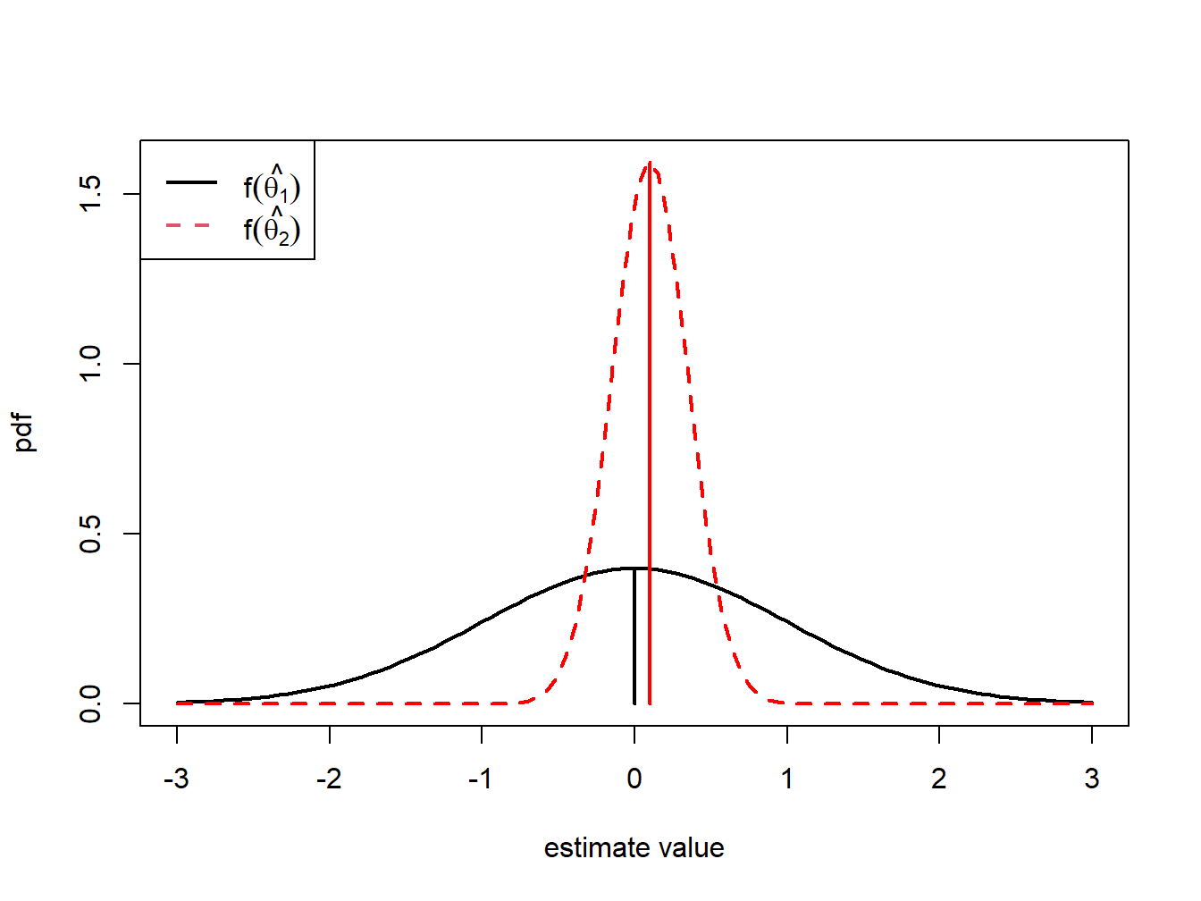
Figure 7.1: Distributions of competing estimators for $\theta=0$. $\hat{\theta}_{1}$ is unbiased but has high variance, and $\hat{\theta}_{2}$ is biased but has low variance.

7.2.2 Precision

An estimate is, hopefully, our best guess of the true (but unknown) value of $\theta$. Our guess most certainly will be wrong, but we hope it will not be too far off. A precise estimate is one in which the variability of the estimation error is small. The variability of the estimation error is captured by the mean squared error.

Definition 7.2 The mean squared error of an estimator $\hat{\theta}$ of $\theta$ is given by: $$\begin{equation} \mathrm{mse}(\hat{\theta},\theta)=E[(\hat{\theta}-\theta)^{2}]=E[\mathrm{error}(\hat{\theta},\theta)^{2}]\tag{7.4} \end{equation}$$

The mean squared error measures the expected squared deviation of $\hat{\theta}$ from $\theta$. If this expected deviation is small, then we know that $\hat{\theta}$ will almost always be close to $\theta$. Alternatively, if the mean squared is large then it is possible to see samples for which $\hat{\theta}$ is quite far from $\theta$. A useful decomposition of $\mathrm{mse}(\hat{\theta},\theta)$ is: $$\mathrm{mse}(\hat{\theta},\theta)=E[(\hat{\theta}-E[\hat{\theta}])^{2}]+\left(E[\hat{\theta}]-\theta\right)^{2}=\mathrm{var}(\hat{\theta})+\mathrm{bias}(\hat{\theta},\theta)^{2}$$ The derivation of this result is straightforward. Use the add and subtract trick and write $$\hat{\theta}-\theta=\hat{\theta}-E[\hat{\theta}]+E[\hat{\theta}]-\theta.$$ Then square both sides giving $$(\hat{\theta}-\theta)^{2}=\left(\hat{\theta}-E[\hat{\theta}]\right)^{2}+2\left(\hat{\theta}-E[\hat{\theta}]\right)\left(E[\hat{\theta}]-\theta\right)+\left(E[\hat{\theta}]-\theta\right)^{2}.$$ Taking expectations of both sides yields,

$$\begin{align*} \mathrm{mse}(\hat{\theta},\theta) & =E\left[\left(\hat{\theta}-E[\hat{\theta}]\right)\right]^{2}+2\left(E[\hat{\theta}]-E[\hat{\theta}]\right)\left(E[\hat{\theta}]-\theta\right)+E\left[\left(E[\hat{\theta}]-\theta\right)^{2}\right]\\ & =E\left[\left(\hat{\theta}-E[\hat{\theta}]\right)\right]^{2}+E\left[\left(E[\hat{\theta}]-\theta\right)^{2}\right]\\ & =\mathrm{var}(\hat{\theta})+\mathrm{bias}(\hat{\theta},\theta)^{2}. \end{align*}$$

The result states that for any estimator $\hat{\theta}$ of $\theta$, $\mathrm{mse}(\hat{\theta},\theta)$ can be split into a variance component, $\mathrm{var}(\hat{\theta})$, and a squared bias component, $\mathrm{bias}(\hat{\theta},\theta)^{2}$. Clearly, $\mathrm{mse}(\hat{\theta},\theta)$ will be small only if both components are small. If an estimator is unbiased then $\mathrm{mse}(\hat{\theta},\theta)=\mathrm{var}(\hat{\theta})=E[(\hat{\theta}-\theta)^{2}]$ is just the squared deviation of $\hat{\theta}$ about $\theta$. Hence, an unbiased estimator $\hat{\theta}$ of $\theta$ is good, if it has a small variance.

The $\mathrm{mse}(\hat{\theta},\theta)$ and $\mathrm{var}(\hat{\theta})$ are based on squared deviations and so are not in the same units of measurement as $\theta$. Measures of precision that are in the same units as $\theta$ are the root mean square error and the standard error.

Definition 2.6 The root mean square error and the standard error of an estimator $\hat{\theta}$ are:

$$\begin{equation} \mathrm{rmse}(\hat{\theta},\theta)=\sqrt{\mathrm{mse}(\hat{\theta},\theta)},\tag{7.5} \end{equation}$$

$$\begin{equation} \mathrm{se}(\hat{\theta})=\sqrt{\mathrm{var}(\hat{\theta})}.\tag{7.6} \end{equation}$$

If $\mathrm{bias}(\hat{\theta},\theta)\approx0$ then the precision of $\hat{\theta}$ is typically measured by $\mathrm{se}(\hat{\theta})$.

With the concepts of bias and precision in hand, we can state what defines a good estimator.

Definition 7.3 A good estimator $\hat{\theta}$ of $\theta$ has a small bias (7.3) and a small standard error (7.6).

7.2.3 Estimated standard errors

Standard error formulas $\mathrm{se}(\hat{\theta})$ that we will derive often depend on the unknown values of the GWN model parameters. For example, later on we will show that $\mathrm{se}(\hat{\mu}) = \sigma^2 / T$ which depends on the GWN parameter $\sigma^2$ which is unknown. Hence, the formula for $\mathrm{se}(\hat{\mu})$ is a practically useless quantity as we cannot compute its value because we don’t the know the value of $\sigma^2$. Fortunately, we can create a practically useful formula by replacing the unknown quantity $\sigma^2$ with an good estimate $\hat{\sigma}^2$ that we compute from the data. This gives rise the estimated asymptotic standard error $\widehat{\mathrm{se}}(\hat{\mu}) = \hat{\sigma}^2 / T$.