9.6 Model Specification Tests
- Review GWN model assumptions
- Discuss why it is interesting and useful to test these assumptions
- What to do if certain assumptions are violated?
9.6.1 Tests for normality
Why do we care about normality?
- Return distribution only depends on mean and volatility (and correlation in multivariate case).
- Justifies volatility as an appropriate measure of risk.
- Gives formula for Value-at-risk calculations.
- Justifies mean-variance portfolio theory and Black-Scholes option pricing formula.
- GWN model parameter estimates and standard error formula do not require the data to be normally distributed. These estimates are consistent and asymptotically normally distributed for many non-normal distributions. There may be estimators that are more accurate (i.e., have smaller standard errors)
What to do if returns are found to not be normally distributed?
- Return distribution characteristics in addition to mean and volatility may be important to investors. Volatility may not be the best measure of asset return risk. For example, skewness and kurtosis. If many returns are non-normal then this casts doubt on the appropriateness of mean-variance portfolio theory.
- Standard practice is to compute VaR based on a normal distribution. If returns are not normally distributed this is an incorrect way to compute VaR. Instead of using the normal distribution quantile to compute VaR you can use the empirical quantile to compute VaR. If returns are substantially non-normal in the tails of the distribution then the empirical quantile will be more appropriate than the normal quantile for computing VaR
- How are returns non-normal? This is important.
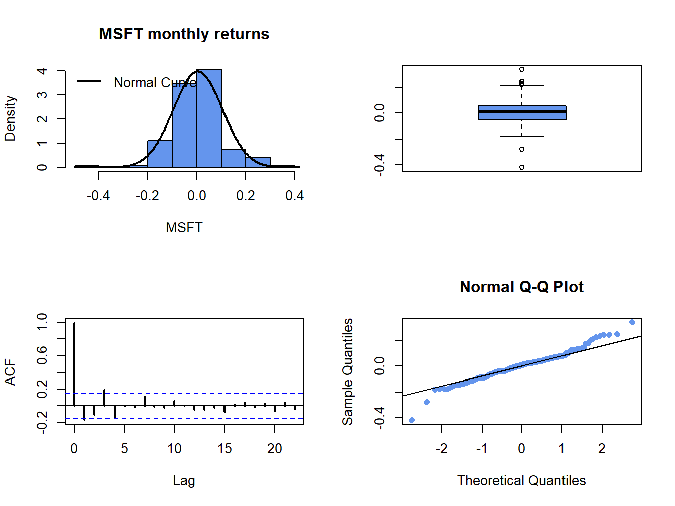
In chapter 5, we used histograms, normal QQ-plots, and boxplots to assess whether the normal distribution is a good characterization of the empirical distribution of daily and monthly returns. For example, Figure 9.2 shows the four-panel plot for the monthly returns on Microsoft that we used to summarize the empirical distribution of returns. The histogram and smoothed histogram show that the empirical distribution of returns is bell-shaped like the normal distribution, whereas the boxplot and normal QQ-plot shows that returns have fatter tails than the normal distribution. Overall, the graphical descriptive statistics suggest that distribution of monthly Microsoft returns is not normally distributed. However, graphical diagnostics are not formal statistical tests. There are estimation errors in the statistics underlying the graphical diagnostics and it is possible that the observed non-normality of the data is due to sampling uncertainty. To be more definitive, we should use an appropriate test statistic to test the null hypothesis that the random return, \(R_{t}\), is normally distributed. Formally, the null hypothesis to be tested is:
\[\begin{equation} H_{0}:R_{t}\, \textrm{is normally distributed}\tag{9.28} \end{equation}\] The alternative hypothesis is that \(R_{t}\) is not normally distributed: \[\begin{equation} H_{1}:R_{t}\,\textrm{is not normally distributed}\tag{9.29} \end{equation}\]
Here, we do not specify a particular distribution under the alternative (e.g., a Student’s t distribution with a 5 degrees of freedom). Our goal is to have a test statistic that will reject the null hypothesis (9.28) for a wide range of non-normal distributions.

Figure 9.2: Four panel distribution plot for Microsoft monthly returns.
9.6.1.1 JB test based on skewness and kurtosis

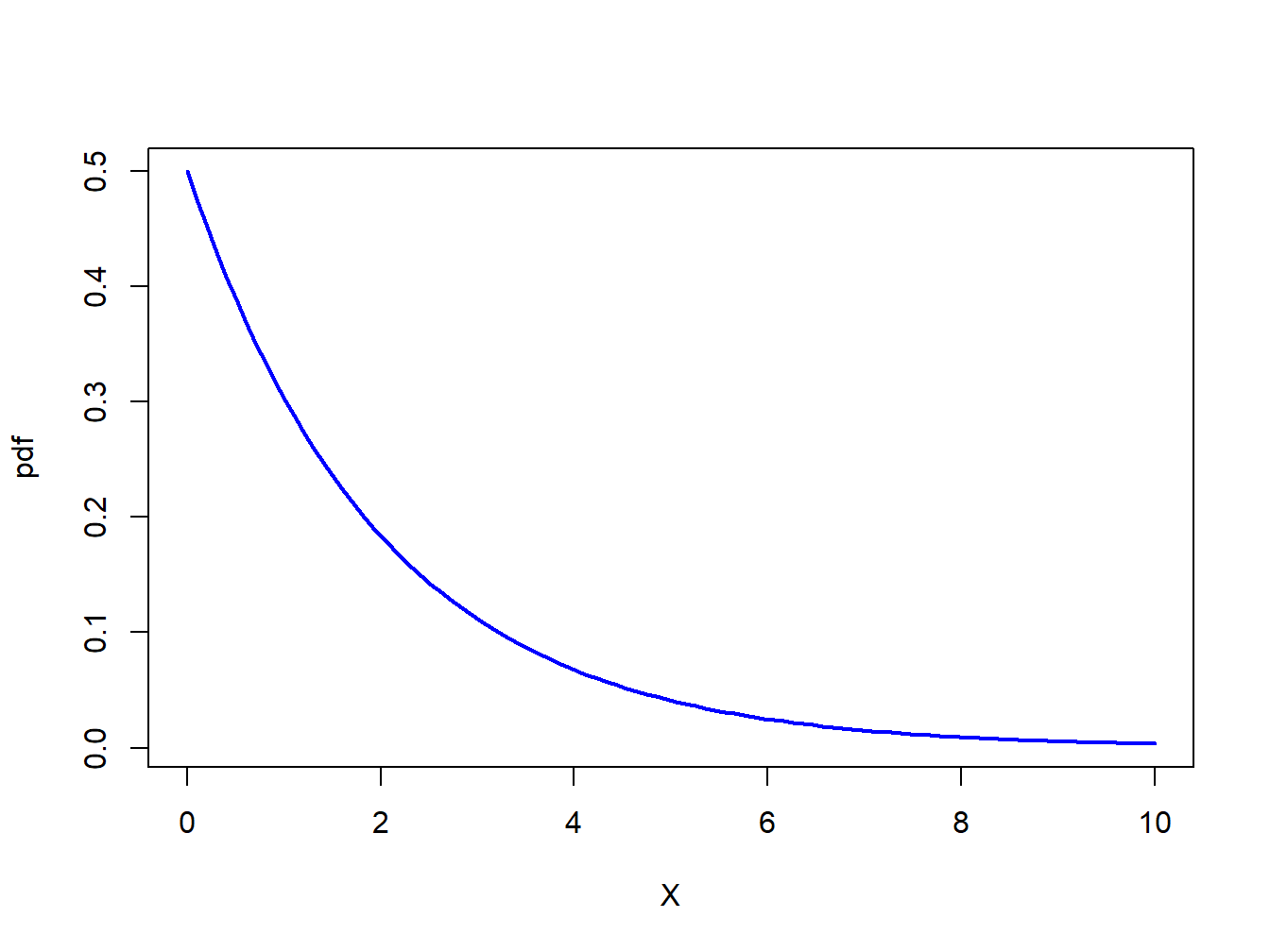
Figure 9.3: pdf of \(\chi^{2}(2)\)
In Chapter 2, we showed that the skewness and kurtosis of a normally distributed random variable are equal to zero and three, respectively. We can use this information to develop a simple test of (9.28) against (9.29) based on testing the hypotheses: \[\begin{eqnarray} H_{0}:\mathrm{skew}(R_{t}) & = & 0\,\,\,\mathrm{and}\,\,\,\mathrm{kurt}(R_{t})=3\,\,vs.\,\,\tag{9.30}\\ H_{1}:\mathrm{skew(}R_{t}) & \neq & 0\,\,\,\mathrm{or}\,\,\,\mathrm{kurt}(R_{t})\neq3\,\,\,\mathrm{or}\,\,\,\mathrm{both}.\tag{9.31} \end{eqnarray}\] To develop a test statistic for testing (9.30) against (9.31), Jarque and Bera (1981) used the result (see Kendall and Stuart, 1977) that if \(\{R_{t}\}\sim\mathrm{iid}\,N(\mu,\sigma^{2})\) then by the CLT it can be shown that: \[ \left(\begin{array}{c} \widehat{\mathrm{skew}}_{r}\\ \widehat{\mathrm{kurt}}_{r}-3 \end{array}\right)\sim N\left(\left(\begin{array}{c} 0\\ 0 \end{array}\right),\left(\begin{array}{cc} \frac{6}{T} & 0\\ 0 & \frac{24}{T} \end{array}\right)\right), \] for large enough \(T\), where \(\widehat{\mathrm{skew}}_{r}\) and \(\widehat{\mathrm{kurt}}_{r}\) denote the sample skewness and kurtosis of the returns \(\{r_{t}\}_{t=1}^{T}\), respectively. This motivates Jarque and Bera’s JB statistic: \[\begin{equation} \mathrm{JB}=T\times\left[\frac{\left(\widehat{\mathrm{ske}w}_{r}\right)^{2}}{6}+\frac{\left(\widehat{\mathrm{kurt}}_{r}-3\right)^{2}}{24}\right],\tag{9.32} \end{equation}\] to test (9.28) against (9.29). If returns are normally distributed then \(\widehat{\mathrm{skew}}_{r}\approx0\) and \(\widehat{\mathrm{kurt}}_{r}-3\approx0\) so that \(\mathrm{JB}\approx0\). In contrast, if returns are not normally distributed then \(\widehat{\mathrm{skew}}_{r}\neq0\) or \(\widehat{\mathrm{kurt}}_{r}-3\neq0\) or both so that \(\mathrm{JB}>0\). Hence, if JB is big then there is data evidence against the null hypothesis that returns are normally distributed.
To determine the critical value for testing (9.28)
at a given significance level we need the distribution of the JB statistic
(9.32) under the null hypothesis (9.28).
To this end, Jarque and Bera show, assuming (9.28)
and large enough \(T\), that:
\[
\mathrm{JB}\sim\chi^{2}(2),
\]
where \(\chi^{2}(2)\) denotes a chi-square distribution with two degrees
of freedom (see Appendix). Hence, the critical values for the JB statistic
are the upper quantiles of \(\chi^{2}(2)\). Figure 9.3
shows the pdf of \(\chi^{2}(2)\). The 90%, 95% and 99% quantiles
can be computed using the R function qchisq():
## [1] 4.61 5.99 9.21Since the 95% quantile of \(\chi^{2}(2)\) is \(5.99\approx6\), a simple rule of thumb is to reject the null hypothesis (9.28) at the 5% significance level if the JB statistic (9.32) is greater than 6.
Let \(X\sim\chi^{2}(2)\). The p-value of the JB test is computed using: \[ p-value=\Pr(X>JB). \] If the p-value() is less than \(\alpha\) then the null () is rejected at the
The sample skewness and excess kurtosis values for the monthly returns on Microsoft, Starbucks, and the S&P 500 index are
##                    MSFT   SBUX SP500
## Skewness        -0.0901 -0.987 -0.74
## Excess Kurtosis  2.0802  3.337  1.07
The sample skewness values for the assets are not too large but the sample excess kurtosis values are fairly large. The JB statistics for the three assets are easy to compute
n.obs = nrow(gwnMonthlyRetC)
JB = n.obs*((as.numeric(skewhat)^2)/6 + (as.numeric(ekurthat)^2)/24)
names(JB) = colnames(gwnMonthlyRetC)
JB
## MSFT SBUX SP500
## 31.2 107.7 23.9Since all JB values are greater than 6, we reject the null hypothesis that the monthly returns are normally distributed.
You can also use the tseries function jarque.bera.test()
to compute the JB statistic:
##
##  Jarque Bera Test
##
## data:  gwnMonthlyRetC[, 1]
## X-squared = 31, df = 2, p-value = 2e-07##
## Jarque Bera Test
##
## data: gwnMonthlyRetC[, 2]
## X-squared = 108, df = 2, p-value <2e-16##
## Jarque Bera Test
##
## data: gwnMonthlyRetC[, 3]
## X-squared = 24, df = 2, p-value = 7e-06The test statistics are slightly different from the direct calculation
above due to differences in how the sample skewness and sample kurtosis
is computed within the function jarque.bera.test().
\(\blacksquare\)
9.6.1.2 Shipiro Wilks test
To be complete…
9.6.2 Tests for no autocorrelation

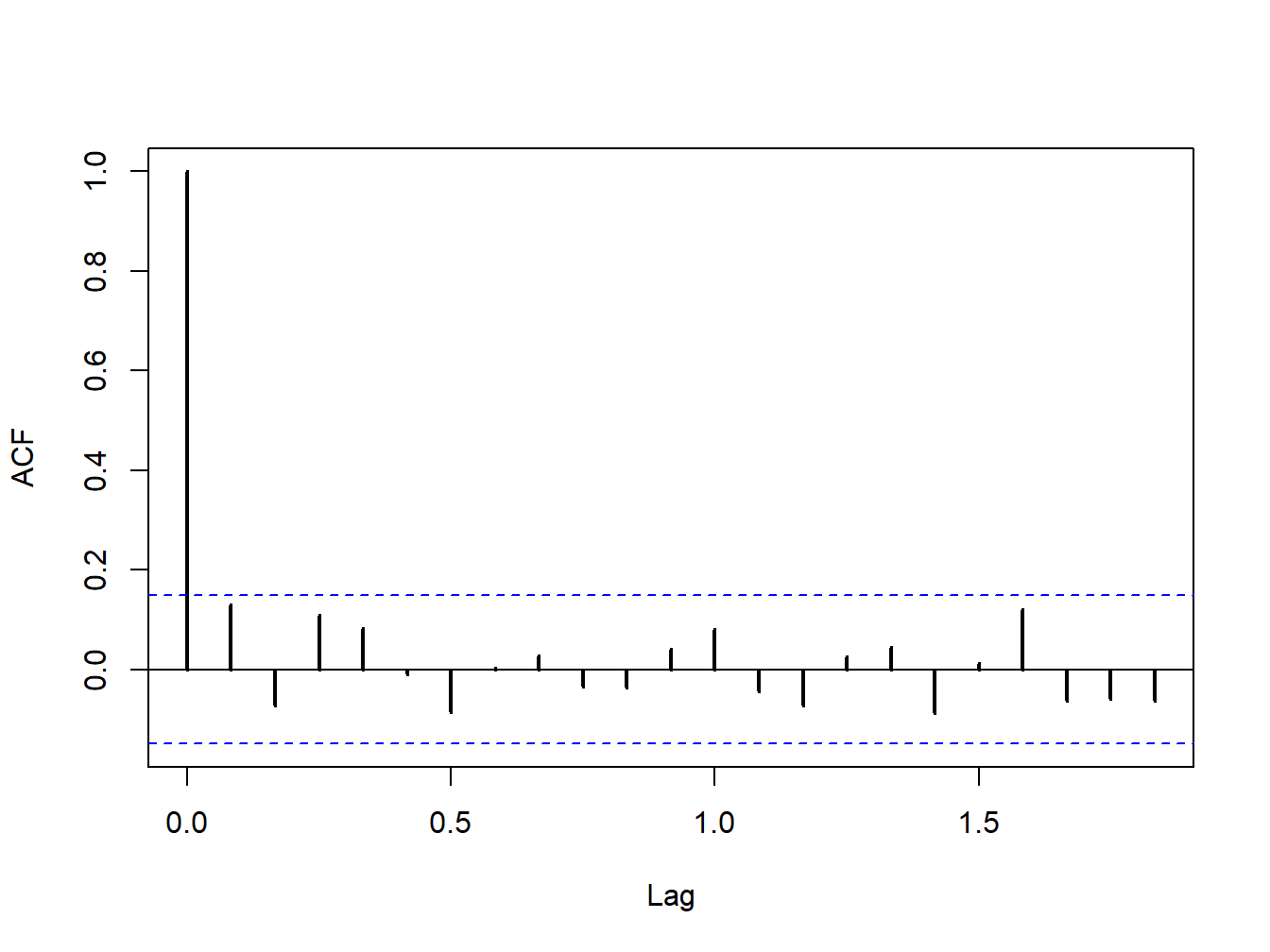
Figure 9.4: SACF for monthly returns on the S&P 500 index.
A key assumption of the GWN model is that returns are uncorrelated over time (not autocorrelated). In efficient financial markets where prices fully reflect true asset value, returns of actively traded assets should not be autocorrelated. In addition, if returns are autocorrelated then they are predictable. That is, future returns can be predicted from the past history of returns. If this is the case then trading strategies can be easily developed to exploit this predictability. But if many market participants act on these trading strategies then prices will adjust to eliminate any predictability in returns. Hence, for actively traded assets in well functioning markets we expect to see that the returns on these assets are uncorrelated over time.
For less frequently traded assets returns may appear to be autocorrelated due to stale pricing.
As we saw in Chapter 6, this allows us to aggregate the GWN model over time and, in particular, derive the square-root-of time rule for aggregating return volatility. If returns are substantially correlated over time (i.e., autocorrelated) then the square-root-of-time rule will not be an accurate way to aggregate volatility.
To measure autocorrelation in asset returns \(\{R_{t}\)} we use the j\(^{th}\) lag autocorrelation coefficient \[\begin{align*} \rho_{j} & =\mathrm{cor}(R_{t},R_{t-j})=\frac{\mathrm{cov}(R_{t},R_{t-j})}{\mathrm{var}(R_{t})}, \end{align*}\] which is estimated using the sample autocorrelation \[ \hat{\rho}_{j}=\frac{\frac{1}{T-1}\sum_{t=j+1}^{T}(r_{t}-\hat{\mu})(r_{t-j}-\hat{\mu})}{\frac{1}{T-1}\sum_{t=1}^{T}(r_{t}-\hat{\mu})^{2}}. \] In chapter 5, we used the sample autocorrelation function (SACF) to graphically evaluate the data evidence on autocorrelation for daily and monthly returns. For example, Figure 9.4 shows the SACF for the monthly returns on the S&P 500 index. Here we see that none of the \(\hat{\rho}_{j}\)values are very large. We also see a pair of blue dotted lines on the graph. As we shall see, these dotted lines are related to critical values for testing the null hypothesis that \(\rho_{j}=0\). Hence, if
9.6.2.1 Individual tests
Individual tests for autocorrelation are similar to coefficient tests discussed earlier and are based on testing the hypotheses \[ H_{0}:\rho_{j}=0\,\,\,vs.\,\,\,H_{1}:\rho_{j}\neq0, \] for a given lag \(j\). The tests rely on the result, justified by the CLT if \(T\) is large enough, that if returns are covariance stationary and uncorrelated then \[\begin{align*} \hat{\rho}_{j}\sim N\left(0,\frac{1}{T}\right)\text{ for all }j\geq1\,\mathrm{and}\,\mathrm{se}(\hat{\rho}_{j})=\frac{1}{\sqrt{T}}. \end{align*}\] This motivates the test statistics \[ t_{\rho_{j=0}}=\frac{\hat{\rho}_{j}}{\mathrm{se}(\hat{\rho}_{j})}=\frac{\hat{\rho}_{j}}{1/\sqrt{T}}=\sqrt{T}\hat{\rho}_{j},\,j\geq1 \] and the 95% confidence intervals \[ \hat{\rho}_{j}\pm2\cdot\frac{1}{\sqrt{T}}. \] If we use a 5% significance level, then we reject the null hypothesis \(H_{0}:\rho_{j}=0\) if \[ |t_{\rho_{j=0}}|=\left\vert \sqrt{T}\hat{\rho}_{j}\right\vert >2. \] That is, reject if \[ \hat{\rho}_{j}>\frac{2}{\sqrt{T}}\text{ or }\hat{\rho}_{j}<\frac{-2}{\sqrt{T}}. \] Here we note that the dotted lines on the SACF are at the points \(\pm2\cdot\frac{1}{\sqrt{T}}\). If the sample autocorrelation \(\hat{\rho}_{j}\) crosses either above or below the dotted lines then we can reject the null hypothesis \(H_{0}:\rho_{j}=0\) at the 5% level.
9.6.2.2 Joint tests
- Have to be careful how to interpret the individual tests. Cannot simply use 20 individual tests at the 5% level to test a joint hypothesis at the 5% level. With independent individual tests each test has a 5% probability of rejecting the null when it is true. So if you do 20 individual tests it would not be surprising if one tests rejects and this could be purely by chance (a type I error) if the null of no autocorrelation was true.
To be complete
9.6.3 Tests for constant parameters
A key assumption of the GWN model is that returns are generated from a covariance stationary time series process. As a result, all of the parameters of the GWN model are constant over time. However, as shown in Chapter 5 there is evidence to suggest that the assumption of covariance stationarity may not always be appropriate. For example, the volatility of returns for some assets does not appear to be constant over time.
A natural null hypothesis associated with the covariance stationarity assumption for the GWN model for an individual asset return has the form: \[ H_{0}:\mu_{i},\sigma_{i},\rho_{ij}\, \text{are constant over time}. \] To reject this null implied by covariance stationarity, one only needs to find evidence that at least one parameter is not constant over time.
9.6.3.1 Formal tests (two parameter structural change)
To be completed
- Do two-sample structural change tests based on known segments. Analysis is very similar to testing equality of parameters across two assets.
9.6.4 Tests for constant parameters based on rolling estimators
In Chapter 5 we introduced rolling descriptive statistics to informally investigate the assumption of covariance stationarity. Given any parameter \(\theta\) of the GWN model (or any function of the parameters), we can compute a set of rolling estimates of \(\theta\) over windows of length \(n<T\): \(\{\hat{\theta}_t(n) \}_{t=n}^{T}\). A time plot of these rolling estimates may show evidence of non-stationary behavior in returns.
However, one must always keep in mind that estimates have estimation error and part of the observed time variation in the rolling estimates \(\{\hat{\theta}_t(n) \}_{t=n}^{T}\) is due to random estimation error. To account for this estimation error, rolling estimates are often displayed with estimated standard error bands of the form:
\[\begin{equation} \hat{\theta}_t(n) \pm c\times \widehat{\mathrm{se}}\left( \hat{\theta}_t(n)\right), \tag{9.33} \end{equation}\]
where \(c\) is a constant representing some multiple of the estimated standard error. Typically, \(c\) is chosen so that (9.33) represents an approximate confidence interval for \(\theta\). For example, setting \(c=2\) gives an approximate 95% confidence interval.
As in Chapter 5, we compute 24-month rolling estimates of \(\mu\) and \(\sigma\) for Microsoft, Starbucks and the S&P 500 index using the zoo function rollapply():
roll.muhat = rollapply(gwnMonthlyRetC, width = 24, by = 1,
                       by.column = TRUE, FUN = mean, align = "right")
roll.sigmahat = rollapply(gwnMonthlyRetC, width = 24, by = 1,
                          by.column = TRUE, FUN = sd, align = "right")
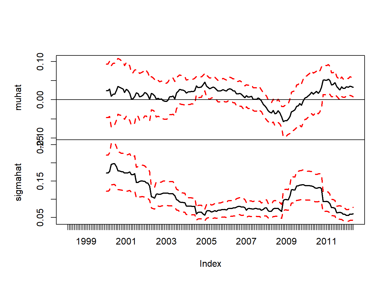
Estimated standard errors for \(\hat{\mu}_t(n)\) and \(\hat{\sigma}_t(n)\) are computed using: \[ \widehat{\mathrm{se}}(\hat{\mu}_t(n)) = \frac{\hat{\sigma}_t(n)}{\sqrt{T}}, ~ \widehat{\mathrm{se}}(\hat{\sigma}_t(n)) = \frac{\hat{\sigma}_t(n)}{\sqrt{2T}} \] Figure 9.5 shows the rolling estimates of \(\mu\) (top panel) and \(\sigma\) (bottom panel) for Starbucks together with 95% confidence intervals (\(\pm2\times\) standard error bands) computed using:
se.muhat.SBUX = roll.sigmahat[, "SBUX"]/sqrt(24)
se.sigmahat.SBUX = roll.sigmahat[, "SBUX"]/sqrt(2 * 24)
lower.muhat.SBUX = roll.muhat[, "SBUX"] - 2 * se.muhat.SBUX
upper.muhat.SBUX = roll.muhat[, "SBUX"] + 2 * se.muhat.SBUX
lower.sigmahat.SBUX = roll.sigmahat[, "SBUX"] - 2 * se.sigmahat.SBUX
upper.sigmahat.SBUX = roll.sigmahat[, "SBUX"] + 2 * se.sigmahat.SBUX
# plot estimates with standard error bands
dataToPlot = merge(roll.muhat[, "SBUX"], lower.muhat.SBUX,
                   upper.muhat.SBUX, roll.sigmahat[,"SBUX"],
                   lower.sigmahat.SBUX, upper.sigmahat.SBUX)
my.panel <- function(...) {
  lines(...)
  abline(h = 0)
}
plot.zoo(dataToPlot, main = "", screens = c(1, 1, 1, 2, 2, 2),
         lwd = 2, col = c("black","red", "red", "black", "red", "red"),
         lty = c("solid", "dashed", "dashed", "solid", "dashed", "dashed"),
         panel = my.panel, ylab = list("muhat", "sigmahat"))
Figure 9.5: 24-month rolling estimates of \(\mu\) and \(\sigma\) for Starbucks with estimated standard error bands
The standard error bands for \(\hat{\mu}_t(n)\) are fairly wide, especially during the high volatility periods of the dot-com boom-bust and the financial crisis. During the dot-com period the 95% confidence intervals for \(\mu\) are wide and contain both positive and negative values reflecting a high degree of uncertainty about the value of \(\mu\). However, during the economic boom around 2005, where \(\hat{\mu}_t(n)\) is large and \(\hat{\sigma}_t(n)\) is small, the 95% confidence interval for \(\mu\) does not contain zero and one can infer that the mean is significantly positive. Also, at the height of the financial crisis, where \(\hat{\mu}_t(n)\) is the largest negative value, the 95% confidence interval for \(\mu\) contains all negative values and one can infer that the mean is significantly negative. At the end of the sample, the 95% confidence intervals for \(\mu\) contain all positive values.52
The standard error bands for \(\hat{\sigma}_t(n)\) are smaller than the bands for \(\hat{\mu}_t(n)\) and one can see more clearly that \(\hat{\sigma}_t(n)\) significantly larger during the dot-com period and the financial crisis period than during the economic boom period and the period after the financial crisis.
\(\blacksquare\)
Plotting rolling estimates with estimated standard error bands is good practice as it reminds you that there is estimation error in the rolling estimates and part of any observed time variation is this estimation error.
We have to be a little careful about interpreting the implicit hypotheses tests underlying the rolling 95% confidence intervals. Each confidence interval represents a single hypothesis test with a 5% significane level. However, we have many confidence intervals and so we are really doing many hypothesis tests. The joint significance level for all of these tests will be larger than the significance level for a single test.↩︎