17.9 Unstandardising: Working backwards
Using the model for tree diameters in Example 17.7 (Aedo-Ortiz et al. 1997) again, suppose now the diameters of the smallest 10% of trees needs to be identified. What are these diameters?
Example 17.9 (Normal distributions backwards) Consider again the trees study. The tree diameters can be modelled with
- a normal distribution; with
- a mean of \(\mu=8.8\) inches; and
- a standard deviation of \(\sigma=2.7\) inches.
This is a different problem than before; previously, the tree diameter was known, so a \(z\)-score could be computed, and hence a probability (Fig. 17.11, top panel). This time, the probability is known, and a tree diameter is sought. That is, working ‘backwards’ is needed (Fig. 17.11, bottom panel), so the \(z\)-tables need to be used ‘backwards’ too.
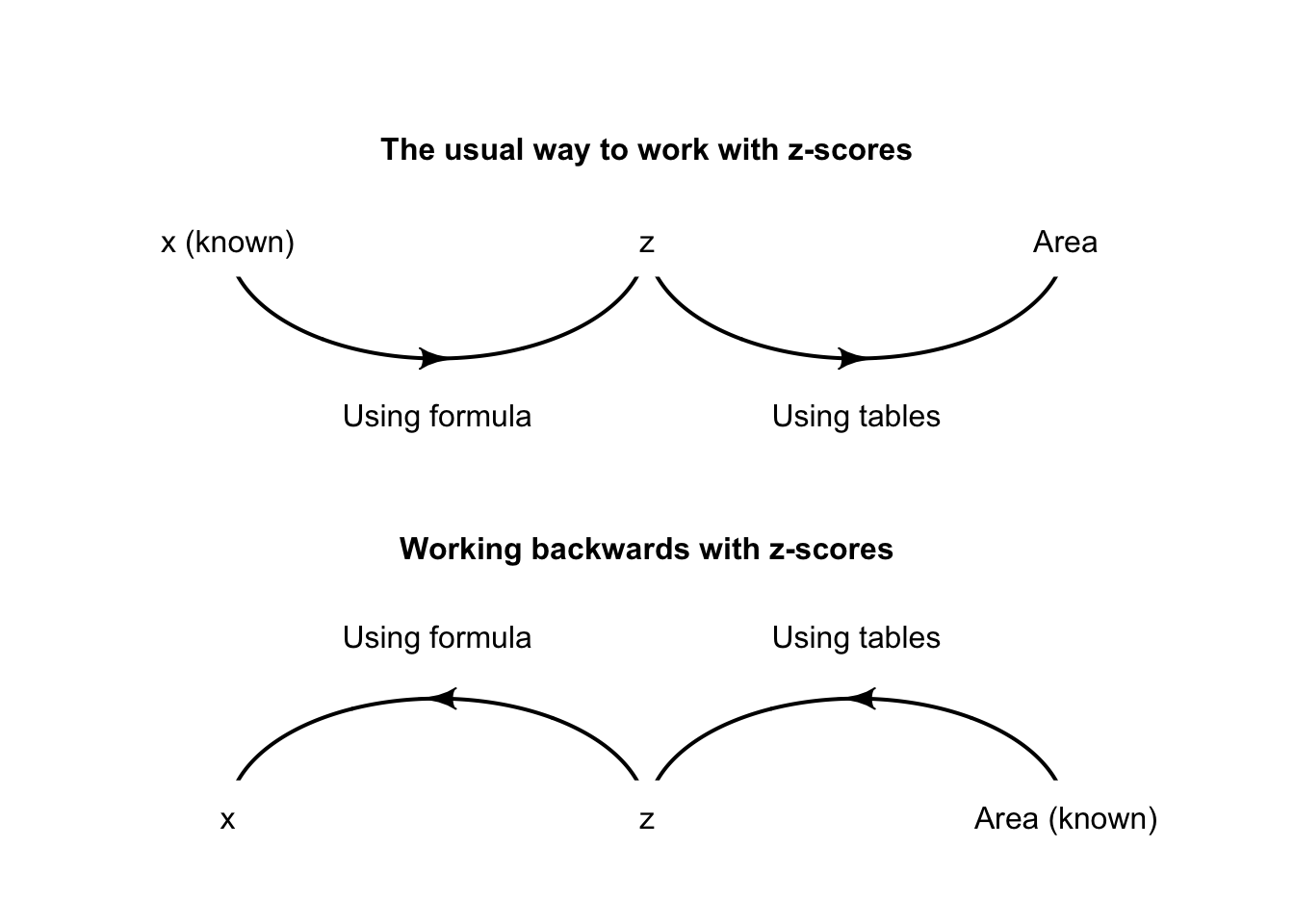
FIGURE 17.11: Working with \(z\)-scores
17.9.1 Using the hard-copy tables
When the \(z\) scores (in the margins of the tables were known, the areas were found in the body of the table. If the area (or probability) is known (found in the body of the table), the corresponding \(z\)-score can be found (in the margins of the table), and hence the observation \(x\); see the animation below. The closest area to 10% in the tables is 0.1003, or 10.03%.
To identify the diameters of the smallest 10% of trees, the \(z\)-score that has an area to the left of 10% (or 0.10) need to be found (at least, as close as possible to 0.10).
17.9.2 Using the online tables
When the area (or probability) is known,
special online tables can be
used (Appendix B.3). In
these tables,
enter the area to the left in search box under Area.to.left,
and the corresponding \(z\)-scores appears under the z.score column
(see the animation below).
Using either the hard-copy or online tables, the appropriate \(z\)-value is \(1.28\) standard deviations below the mean (Fig. 17.12). Then, the \(z\)-score can be converted to an observation value \(x\) using the unstandardising formula6:
\[ x = \mu + z\sigma. \] Using this unstandardising formula:
\[\begin{align*} x &= \mu + (z\times\sigma) \\ &= 8.8 + (-1.28 \times 2.7) = 5.344; \end{align*}\] that is, about 10% of trees have diameters less than about 5.3 inches.
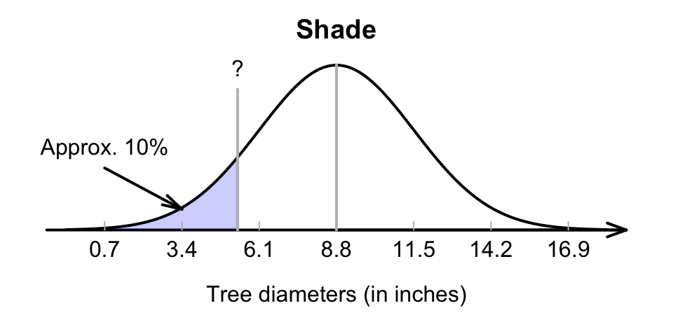
FIGURE 17.12: Tree diameters: The smallest 10%
Definition 17.2 (Unstandardizing formula) When the \(z\)-score is known, the corresponding value of the observation \(x\) is
\[\begin{equation} x = \mu + z\sigma. \tag{17.2} \end{equation}\] This is called the unstandardising formula.Example 17.10 (Normal distributions backwards) Using the model for tree diameters in Example 17.7 (Aedo-Ortiz et al. 1997) again, suppose now the diameters of the largest 25% of trees needs to be identified. What are these diameters?
The tree diameters can be modelled with
- a normal distribution; with
- a mean of \(\mu=8.8\) inches; and
- a standard deviation of \(\sigma=2.7\) inches.
Again, we need to work ‘backwards’ (Fig. 17.13, bottom panel), so the \(z\)-tables need to be used ‘backwards’ too. The largest 25% implies large trees, so we would expect a diameter larger than the mean.
Using a diagram is important (Fig. 17.13): the tables work with the area to the left of the value of interest, which is 75%.
Using either the hard-copy or online tables, the appropriate \(z\)-value is \(z = 0.674\). Then, the \(z\)-score can be converted to an observation value \(x\) using the unstandardising formula:
\[\begin{align*} x &= \mu + (z\times\sigma) \\ &= 8.8 + (0.674 \times 2.7) = 10.621; \end{align*}\] that is, about 25% of trees have diameters larger than about 10.6 inches.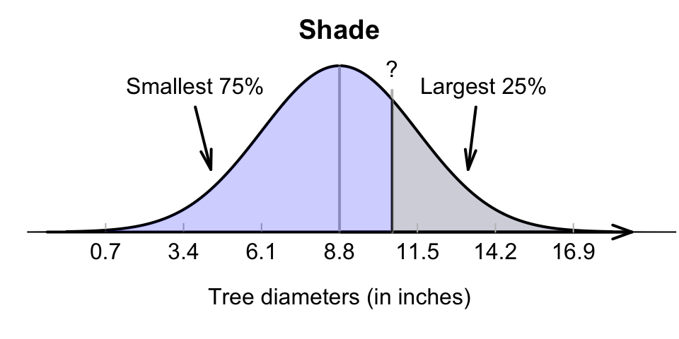
FIGURE 17.13: Tree diameters: The largest 25% is the same as the smallest 75%