13.3 Computing the variation
For quantitative data, the amount of variation in the bulk of the data should be described. Many ways exist to measure the variation in a data set, including:
- The range: very simple and simplistic, so not often used.
- The standard deviation: commonly used.
- The interquartile range (or IQR): commonly used.
- Percentiles: sometimes used.
As always, a value computed from the sample (the statistic) estimates the unknown value in the population (the parameter). Knowing which measure of variation to use is important.
13.3.1 Computing the variation: Range
The range is the simplest measure of variation.
The range is not often used, because only the two extreme observations are used, so it is highly influenced by outliers. Sometimes, the range may be given by stating both the maximum and the minimum value in the data instead of giving the difference between the maximum and the minimum values. The range is measured in the same measurement units as the data.
Example 13.5 (The range) For Jersey cow data
(Example 13.2),
the range is:
\[
\text{Range} = \overbrace{6.5}^{\text{largest}} - \overbrace{4.5}^{\text{smallest}} = 2.0 \text{ percent}.
\]
So the sample median percentage butterfat is 5.20 percent, with a range of 2.00 percent.
13.3.2 Computing the variation: Standard deviation
The population standard deviation is denoted by \(\sigma\) (‘sigma,’ the parameter) and is estimated by the sample standard deviation \(s\) (the statistic). The standard deviation is the most commonly-used measure of variation, but is complicated to compute manually (but you don’t need to do it manually!). The standard deviation is (roughly) the mean distance that the observations are away from the mean. This seems like a reasonable way to measure the amount of variation in some data.
The sample standard deviation \(s\) is mostly found using computer software (e.g., jamovi or SPSS) or a calculator (in Statistics Mode).
You do not have to use the formula to calculate \(s\), but we will demonstrate for those who might find it useful to understand exactly what \(s\) calculates. The formula is:
\[ s = \sqrt{ \frac{\sum(x - \bar{x})^2}{n-1} }, \] where \(\bar{x}\) is the sample mean, \(x\) represents the data values, and \(n\) is the sample size. To use the formula, follow these steps:
- Calculate the sample mean: \(\overline{x}\);
- Calculate the deviations of each observation \(x\) from the mean: \(x-\bar{x}\);
- Square these deviations (to make them all positive values): \((x-\bar{x})^2\);
- Add these values: \(\sum(x-\bar{x})^2\);
- Divide the answer by \(n-1\);
- Take the (positive) square root of the answer.
Example 13.6 (Standard deviation) For the Jersey cow data (Example 13.2), the deviations of each observation from the mean of \(5.25\) can be found (Fig. 13.4). Then follow the steps outlined. You don’t have to do this manually! From Fig. 13.4, the sum of the squared distances is 2.7650. Then, the sample standard deviation is:
\[ s = \sqrt{\frac{2.765}{10-1}} = \sqrt{ 0.3072222} = 0.5542763. \] The sample mean percentage butterfat is 5.25 percent, with a sample standard deviation of 0.554 percent.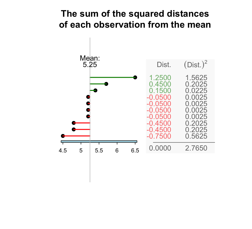
FIGURE 13.4: The standard deviation is related to the sum of the squared-distances from the mean
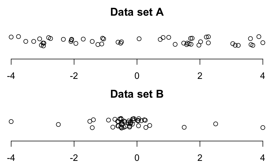
FIGURE 13.5: Dotplots of two sets of data
The sample standard deviation is:
- Positive (unless all observations are the same, when it is zero: there is no variation);
- Best used for (approximately) symmetric data;
- Usually quoted with the mean;
- The most commonly-used measure of variation;
- Measured in the same units as the data;
- Influenced by skewness and outliers, like the mean.
The population standard deviation is unknown. The best estimate is the sample standard deviation: \(s=0.554\)%.
13.3.3 Computing the variation: IQR
The standard deviation uses the value of \(\bar{x}\), so is affected by skewness like the sample mean. Another measure of variation that is not affected by skewness is the inter-quartile range, or IQR. To understand the IQR, understanding quartiles first is important.
Definition 13.7 (Quartiles) Quartiles to describe the variation and shape of data:
- The first quartile \(Q_1\) is a value that separates the smallest 25% of observations from the largest 75%. The \(Q_1\) is like the median of the smaller half of the data, halfway between the minimum value and the median.
- The second quartile \(Q_2\) is a value that separates the smallest 50% of observations from the largest 50%. (This is the median.)
- The third quartile \(Q_3\) is a value that separates the smallest 75% of observations from the largest 25%. The \(Q_3\) is like the median of the larger half of the data, halfway between the median and the maximum value.
Quartiles divide the data into four parts of approximately equal numbers of observations, and a boxplot is a picture of the quartiles. The inter-quartile range, or the IQR is the difference between \(Q_3\) and \(Q_1\). The IQR measures the range of the middle 50% of the data, and is a measure of variation not influenced by outliers. The IQR is measured in the same measurements units as the data.
Quartiles were previously discussed in the context of boxplots (Sect. 12.4.3). For example, a boxplot of the egg-krill data (Greenacre 2016) was shown in Example 12.12; the data are repeated in Table 13.5, and the boxplot in Fig. 13.6.
| 0 | 18 | 0 | 18 |
| 0 | 21 | 0 | 21 |
| 1 | 26 | 0 | 26 |
| 1 | 30 | 0 | 30 |
| 3 | 35 | 1 | 35 |
| 8 | 48 | 1 | 48 |
| 8 | 50 | 1 | 50 |
| 12 | 2 |
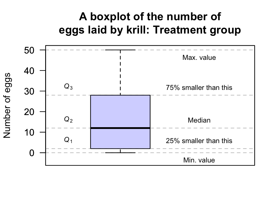
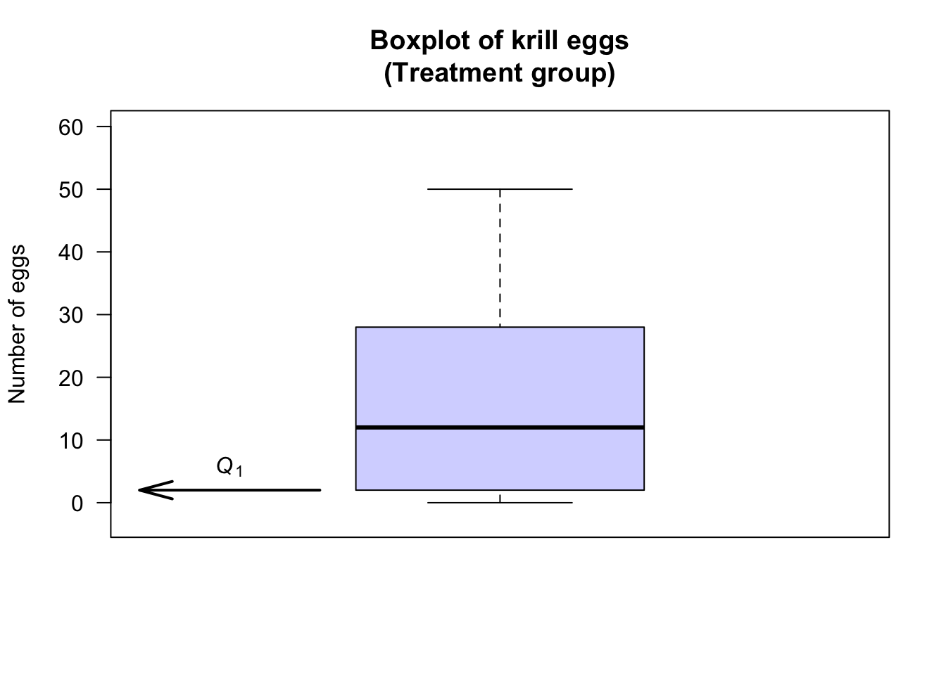
FIGURE 13.6: A boxplot for the krill-egg data; the boxplot just for the treatment group
For the Treatment group:
- 75% of the observations are smaller than about 28, and this is represented by the line at the top of the central box. This is \(Q_3\), or the third quartile.
- 50% of the observations are smaller than about 12, and this is represented by the line in the centre of the central box. This is \(Q_2\), the second quartile or the median.
- 25% of the observations are smaller than about 2, and this is represented by the line at the bottom of the central box. This is \(Q_1\), the first quartile.
The IQR is \(Q_3 - Q_1\) = \(28 - 2\), so that \(\text{IQR} = 26\). The animation below shows how the IQR is found.
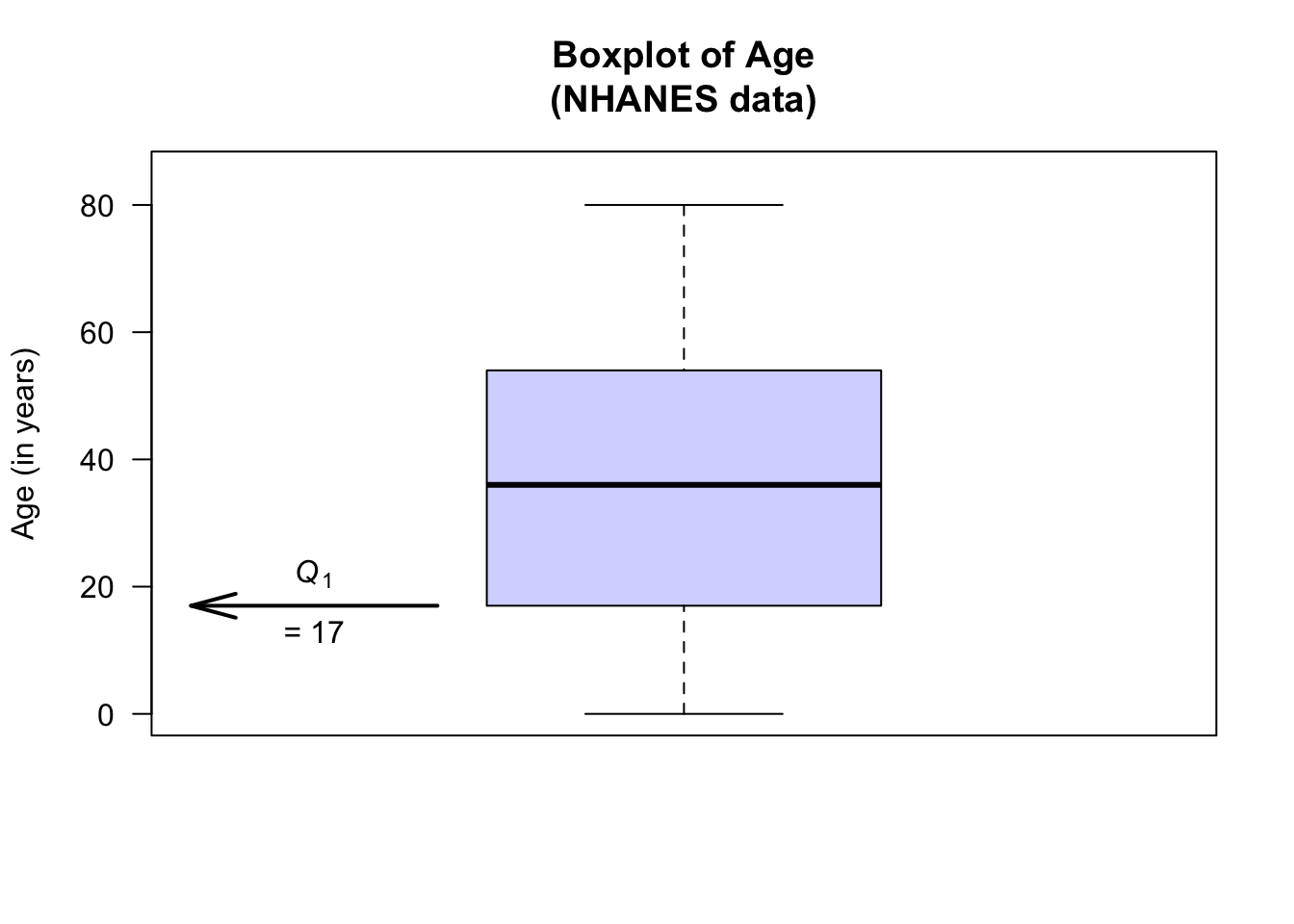
The boxplot for the age of respondents in the NHANES data set is as shown below. For these data:
- No outliers are identified.
- The oldest person is 80.
- About 75% of the subjects are aged less than about 54 (\(Q_3\)): the third quartile \(Q_3 = 54\), the median of the largest half of the data.
- About 50% of the subjects are aged less than about 36 (\(Q_2\), the median): the second quartile \(Q_2 = 36\), the median of the data set.
- About 25% of the subjects are aged less than about 17 (\(Q_1\)): the first quartile \(Q_1 = 17\), the median of the smallest half of the data.
- The youngest subject is aged 0.
Then, \(Q_3 = 54\) and \(Q_1 = 17\), so the \(\text{IQR} = Q_3 - Q_1 = 54 - 17 = 37\) years. The middle 50% of the participants have an age range of 37 years.
13.3.4 Computing the variation: Percentiles
Percentiles can be computed, which are similar to quantiles; for example:
- The 12th percentile is a value separating the smallest 12% of the data from the rest.
- The 67th percentile is a value separating the smallest 67% of the data from the rest.
- The 94th percentile is a value separating the smallest 94% of the data from the rest.
Percentiles are measured in the same measurements units as the data.
By this definition, the first quartile \(Q_1\) is also the 25th percentile, the second quartile \(Q_2\) is also the 50th percentile (and the median), and the third quartile \(Q_3\) is also the 75th percentile.
Percentiles are especially useful for very skewed data and in certain applications. For instance, scientists who monitor rainfall and stream heights, and engineers who use this information, are more interested in extreme weather events rather than the ‘average’ event. Engineers, for example, may design structures to withstand 1-in-100 year events (the 99th percentile) or similar, which are unusual events.
13.3.5 Which measure of variation to use?
Which is the ‘best’ measure of variation for quantitative data? As with measures of location, it depends on the data.
Since the standard deviation calculation uses the mean, it is impacted in the same way as the mean by outliers and skewness, so the standard deviation is best used with approximately symmetric data. The IQR is best used when data are skewed or asymmetric. Sometimes, both the standard deviation and the IQR can be quoted.