14.1 Proportions and percentages
14.1.1 Introduction
In a study by Charig et al. (1986), the aim was to:
…compare (two) different methods of treating renal calculi… to establish which was the most […] successful.
— Charig et al. (1986), p. 879

(Renal calculi are better known as kidney stones.) Data were collected from 700 UK patients, on two qualitative variables:
- The treatment method used (‘A’ or ‘B’): The explanatory variable. Each treatment was used on 350 patients.
- The result (‘success’ or ‘failure’ of the procedure): The response variable.
Both variables are qualitative with two levels. Treatment A was used from 1972–1980, and Treatment B from 1980–1985; that is, the treatments were not randomly allocated, and so confounding may be an issue. For this reason, the researchers also recorded the size of the kidney stone (also a qualitative variable) as a possible confounding variable, as ‘small’ or ‘large.’
Firstly, consider just the small stones (Julious and Mullee 1994). The data can be compiled using a two-way table (Table 14.1), and graphed using a side-by-side or stacked bar chart, for example.
| Success | Failure | Total | |
|---|---|---|---|
| Method A | 81 | 6 | 87 |
| Method B | 234 | 36 | 270 |
Qualitative data can be numerically summarised by computing proportions or percentages. These can be computed:
These are demonstrated within each section, and in a separate Example.
14.1.2 Overall proportions and percentages
From Table 14.1, the overall sample proportion of successes (denoted \(\hat{p}\)) is:
\[\begin{align*} \hat{p} &= \frac{\text{Number of successes}}{\text{Number of procedures}}\\ &= \frac{81 + 234}{6 + 81 + 36 + 234} = 0.882. \end{align*}\] The sample proportion of successful procedures for small kidney stones is 0.882. Sample proportions are denoted using \(\hat{p}\). The sample proportion (a statistic) is an estimate of the unknown population proportion (a parameter), which is denoted \(p\).
The proportion could also be expressed as a percentage:
\[ 0.882 \times 100 = 88.2\%. \] The sample percentage of successful procedures for small kidney stones is 88.2%. The sample proportion and sample percentage are both statistics

Notice that, when computing percentages and proportions, we divide the relevant number by the total number relevant to the context.
14.1.3 Row proportions and percentages
For the small kidney stones (Table 14.1), row proportions (or percentages), and column proportions (or percentages), can be computed
The row proportions (Table 14.2) give the proportion of successes for each Method, since the rows contain the counts for Method A and Method B. Row proportions allow the proportions within the rows to be compared: \(81 \div 87 = 0.931\) (or 93.1%) of operations in the sample were successful for Method A, and \(0.867\) (or 86.7%) of operations were successful in the sample for Method B. This suggests that, for small kidney stones, Method A is more successful than Method B in the sample.
| Success | Failure | Total | |
|---|---|---|---|
| Method A | 93.1 | 6.9 | 100 |
| Method B | 86.7 | 13.3 | 100 |
14.1.4 Column proportions and percentages
For the small kidney stones (Table 14.1), column proportions can also be computed (Table 14.3). The column proportions give the proportion of successes within each method (since the columns contain the procedure results). Column proportions allow the proportions (or percentages) within columns to be compared: \(81 \div (81 + 234) = 0.257\) (or 25.7%) of all successful operations came from using Method A, and \(0.143\) (or 14.3% ) failures came from using Method A.
| Success | Failure | |
|---|---|---|
| Method A | 25.7 | 14.3 |
| Method B | 74.3 | 85.7 |
| Total | 100.0 | 100.0 |
While both row and column proportions (or percentages) can be computed, row percentages seems more intuitive here: they compare the success percentage for each treatment method.
14.1.5 Example: Large kidney stones
The data in Table 14.1 are for small kidney stones. Data were also recorded for the large kidney stones (Table 14.4).
For both small and large stones, the success proportions can be computed for Methods A and B (i.e., row percentages), and hence the better method (in the sample) can be identified.
| Success | Failure | Total | |
|---|---|---|---|
| Method A | 192 | 71 | 263 |
| Method B | 55 | 25 | 80 |
Think 14.1 (Percentages) The success proportion for Method A is greater than the success proportion for Method B for small stones (Table 14.1). Now, compute the success proportions for the large stones too (Table 14.4):
- For large stones, the success proportion with Method A is:
- For large stones, the success proportion with Method B is:
Method A has a higher success proportion in the sample for both small (0.931 vs 0.867) and large kidney stones (0.730 vs 0.688). Perhaps the data for small (Table 14.1) and large kidney stones (Table 14.4) can therefore be combined, to produce a single two-way table of just Method and Result (Table 14.5), ignoring size.
| Success | Failure | Total | |
|---|---|---|---|
| Method A | 273 | 77 | 350 |
| Method B | 289 | 61 | 350 |
In summary, the sample shows that:
- For small stones (Table 14.1), Method A has a higher success proportion: Method A: 0.93; Method B: 0.87
- For large stones (Table 14.4), Method A has a higher success proportion: Method A: 0.73; Method B: 0.69
- Combining all stones together (Table 14.5),
Method B has a higher success proportion:
Method A: 0.78; Method B: 0.83
That seems strange… Method A performs better for small and for large kidney stones, but Method B performs better when combined (and size is ignored).
The size of the stone is a confounding variable (Fig. 14.1): The size of the stone is related to success proportion (small stones have a greater success proportion) and the size of the stone is related to the method used (small stones are treated more often with Method B).
This confounding could have been avoided by randomly allocating a treatment methods to patients. However, random allocation was not possible in this study, so the researchers used a different method to manage confounding: recording the size of the kidney stones (and other variables also: the age and sex of the patient); see Sect. 8.2.3.
In this example, acknowledging the size of the kidney stone is important, otherwise the wrong (opposite) conclusion is reached: one would think that Method B is better if the size of the stones was ignored, when the best method really is Method A.
This is called Simpson’s paradox. If the size of the kidney stone had not been recorded, size would have been a lurking variable, and the incorrect conclusion would have been reached.
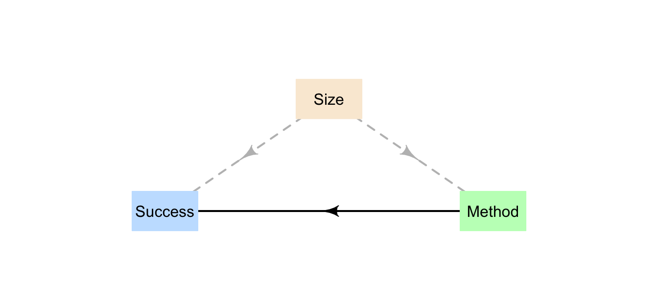
FIGURE 14.1: The size of the stones is related to both the success percentage and the method