12.3 One qualitative variable
For qualitative data, graphs show how often each level of the variable occurs in the data. The three options for graphing qualitative data are:
- Dot chart: Usually a good choice.
- Bar chart: Usually a good choice.
- Pie chart: Only useful in special circumstances, and can be harder to interpret.
Comparing these graphs is useful too; indeed, sometimes a graph may not even be needed.
For nominal data, the order in which the levels of the variables appear is unimportant, so categories could be ordered alphabetically, by size, by personal preference, or any other way. Since you have a choice, think about the order that is most useful to readers. For ordinal data, the natural order of the levels should almost always be used.
Sometimes these graphs are also used for discrete quantitative data with a small number of possible options.
12.3.1 Dot charts (qualitative data)
Dot charts indicate the counts (or the corresponding percentages) in each level, using dots on a line starting at zero. The levels can be on the horizontal or vertical axis; placing the level names on the vertical axis often makes for easier reading, and room for long labels.
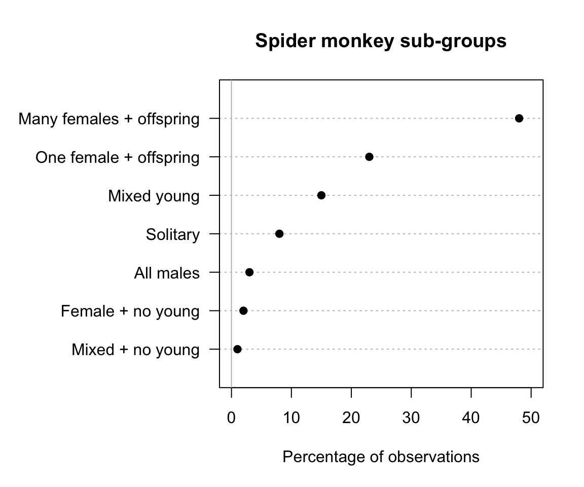
FIGURE 12.8: Dot chart of spider monkey family groups
12.3.2 Bar charts
Bar charts indicate the counts in each category using a bar starting from zero. As with dot charts, the levels can be on the horizontal or vertical axis, but placing the level names on the vertical axis often makes for easier reading, and room for long labels.
Example 12.9 (Bar charts) In a study of functional independence (Ocepek et al. 2013), the type of diagnoses were graphed using a bar chart (Fig. 12.9). For example, two people in the sample have cerebral palsy.
The reason for the different coloured bars becomes apparent in Sect. 12.3.3.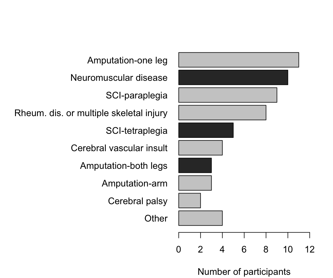
FIGURE 12.9: Diagnoses of participants
For bar charts and dot charts:
- Place the qualitative variable on the horizontal or vertical axis (and label with the levels of the variable).
- Use counts or percentages on the other axis.
- For nominal data, dots and bars can be ordered any way: Think about the most helpful order.
- Bars have gaps between bars, as the bars represent distinct categories. In contrast, the bars in histograms are butted together (except when an interval has a count of zero), as the bars represent a numerical scale.
12.3.3 Pie charts
In pie charts, a circle is divided into segments proportional to the number in each level of the qualitative variable.
Example 12.10 (Pie charts) In a study of functional independence (Ocepek et al. 2013), the severity of the diagnoses were graphed using a pie chart (Fig. 12.10). This picture actually conveys one thing only (“69% of patients had a less severe injury”), so a graph of any kind is probably unnecessary.
The pie chart colours explain the colours used in the bar chart in Example 12.9. This is called encoding extra information into the bar chart.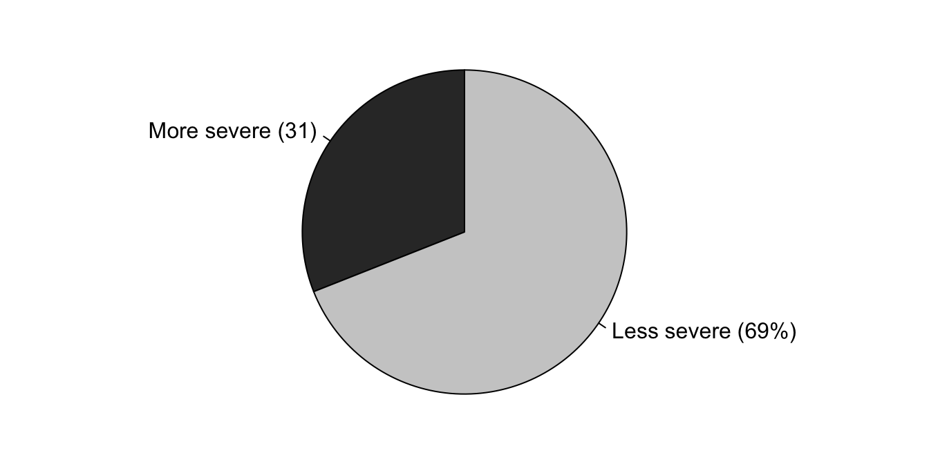
FIGURE 12.10: Severity of diagnoses of participants
Pie charts presents challenges:
- Pie charts only work when graphing parts of a whole.
- Pie charts only work when all options are present (‘exhaustive’).
- Pie charts only work when each unit can appear in just one group (‘mutually exclusive’).
- Pie charts are difficult to use when levels with zero counts, or small counts, are present.
- Pie charts are difficult to read when many categories are present.
- Pie charts are hard to read: In general, human brains are better at comparing lengths (as used in bar and dot charts) than comparing angles (as used in pie charts) (Friel et al. 2001).
Think 12.2 (Pie charts) In which of these situations is a pie chart appropriate?
- The percentage of people who use these web browsers: Firefox, Chrome, and Safari.
- For each state of Australia, the percentage of people who own an iPhone.
- The percentage of students awarded different grades in this course last semester.
A pie chart is not suitable.
Each individual (person) has information recorded on two qualitative variables:
- which browser is being asked about (three levels); and
- whether or not they use that browser (‘yes’ or ‘no’).
The three browsers are not mutually exclusive (people can use more than one of these browsers) nor exhaustive (some people may use browsers not listed, such as Edge, Brave, Vivaldi, etc.). For example, the percentages could be that 65% use Firefox, 84% use Chrome, and 20% use Safari. These add to more than 100%.
A pie chart is not suitable, as the percentages are not parts of a whole.
Again, each individual (person) has information recorded on two qualitative variables:
- which state the person lives in (many levels); and
- whether or not they own an iPhone (‘yes’ or ‘no’).
For example, the percentages could be 53% in Queensland, 61% in NSW, 41% in Victoria, and so on. They could possibly add to more than 100%.
A pie chart is suitable.
Only one qualitative variable is recorded for each individual (person): their grade.
12.3.4 Comparing pie charts and bar charts
Consider the pie chart (using data in Andersen (1977)) in the top panel of Fig. 12.11.
The pie chart displays the number of lung cancer deaths in Fredericia between 1968 and 1971 inclusive, for various age groups (qualitative).
A pie chart is appropriate: only one variable is recorded on each individual (the age of each individual person), and the counts are parts of a whole. However, notice that determining which age groups have the most lung cancer deaths is hard.
The equivalent bar chart (lower panel) makes the comparison easy: clearly the age groups ‘65 to 69’ and ‘Over 74’ have slightly fewer deaths than the other age groups.
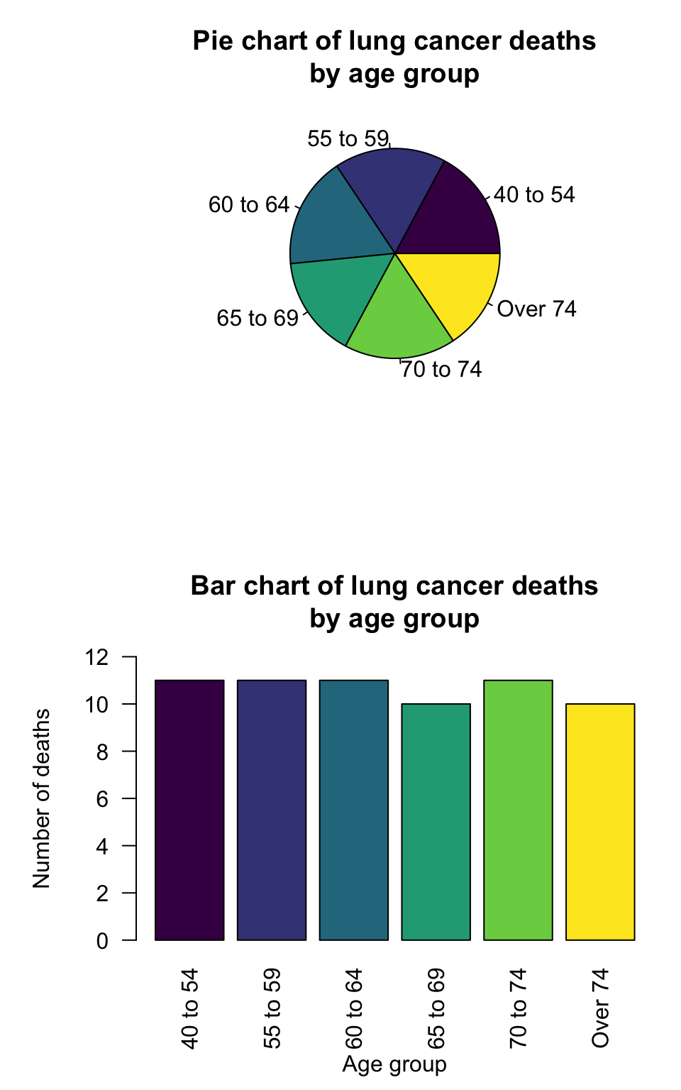
FIGURE 12.11: Graphs from a study of hospital admission of children with asthma
Recall that the purpose of a graph is to is to display information in the clearest, simplest possible way, to help the reaader understand the message(s) in the data. Adding an artificial third dimension usually makes the message hard to see (Siegrist 1996); see Example 12.11.
Example 12.11 (Comparing graphs) In the NHANES study (Center for Disease Control and Prevention (CDC) 1988--1994), the age of each participant was recorded.
Rank the age groups from largest group to smallest group using each graph in Fig. 12.12, all constructed from the same data.
Which graph makes it easiest to compare the sizes of the categories?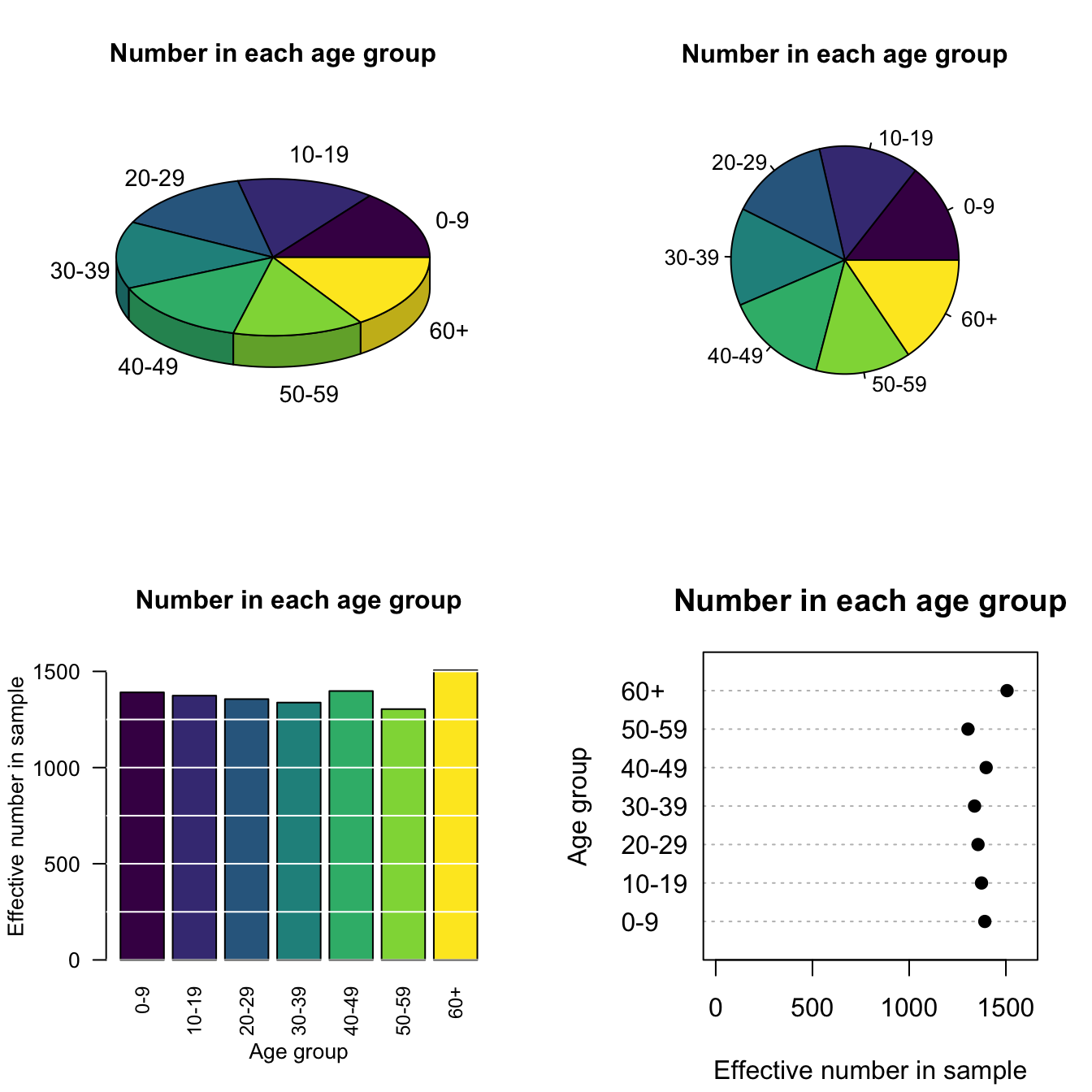
FIGURE 12.12: Four different graphs for the same data
12.3.5 Is a graph needed?
Although graphs are excellent for summarising data, sometimes a graphic is not the best way to display information, especially for qualitative data. Sometimes just writing the information is better (‘69% of diagnoses were less severe’; Fig. 12.10).
Sometimes a table may be better, such as when a small number of levels is present, or if the details are important. Compare different ways of presenting the NHANES age data in Example 12.11: Fig. 12.12 and Table 12.1 display the same data. Which do you think is ‘best,’ and why?
| Age group | Number | Percentage |
|---|---|---|
| 0-9 | 1391 | 14.4 |
| 10-19 | 1374 | 14.2 |
| 20-29 | 1356 | 14 |
| 30-39 | 1338 | 13.8 |
| 40-49 | 1398 | 14.5 |
| 50-59 | 1304 | 13.5 |
| 60+ | 1506 | 15.6 |