13.5 Identifying outliers

Outliers are ‘unusual’ observations: observation quite different (larger or smaller) than the bulk of the data. Deciding whether or not an observation is ‘unusual’ is arbitrary, so ‘rules’ for identifying outliers are somewhat arbitrary too.
Two rules for identifying outliers are:
- The standard deviation rule, useful when the data have an approximately symmetric distribution.
- The IQR rule, useful in other situations.
Understanding the first rule requires studying bell-shaped distributions first. Knowing which rule to use is important.
13.5.1 Bell-shaped (normal) distributions and the 68–95–99.7 rule
To begin, identifying outliers will be studied for data approximately symmetrically distributed. More specifically, symmetric distributions with a bell shape will be studied. For example, the heights of husbands in the UK (Badiou et al. 1988; Hand et al. 1996) have an approximate bell shape (Fig. 13.8, left panel). Most men are between 160 and 185cm; a few are shorter than 160cm and a few taller than 185cm. More formally, bell-shaped distributions are called normal distributions.
These data are from a sample. Of course, every sample is likely to contain different men, and every sample of men will produce a slightly different histogram.
For convenience then, histograms may be smoothed, so that the smoothing produces a shape that represents an ‘average’ of all these possible sample histograms (in other words, an estimate of how the heights may be distributed in the population). For example, see the animation below. The solid line represents the average of many sample histograms.
The smoothed histogram can be drawn can be considered as representing 100% of the observations; after all, every husband in the sample has a height, so is represented somewhere in the histogram. When we do this, the areas under the normal curve are theoretical percentages of the total number.
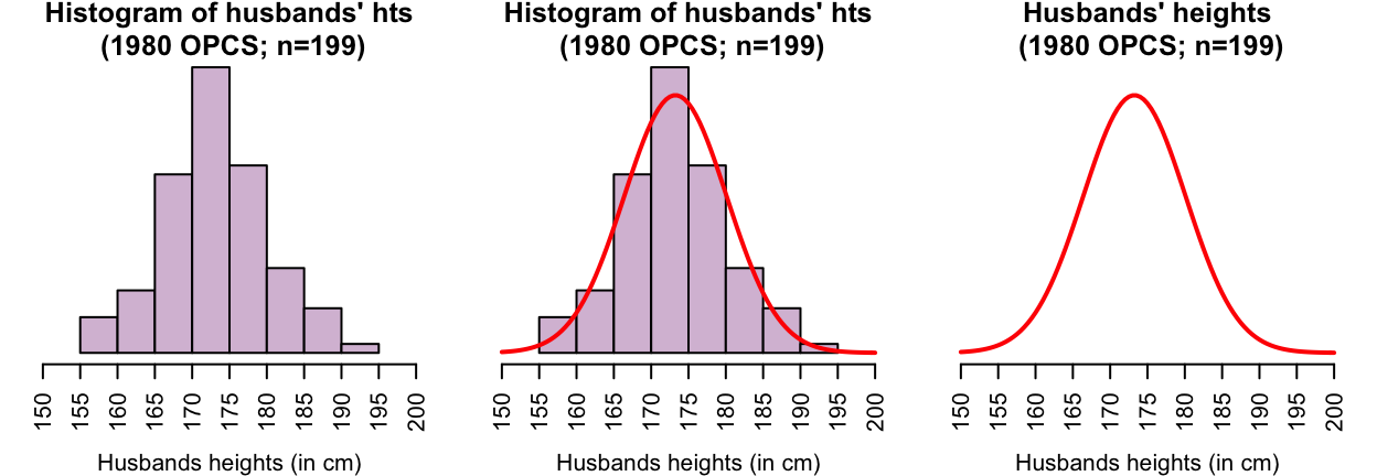
FIGURE 13.8: The heights of husbands have an approximate normal distribution
The smoothed histogram represents all of the husbands’ heights (that is, 100%). Using this idea, areas of the histogram can be shaded (Fig. 13.9) to represent various percentages of the husbands’ heights. For example:
- The middle 50% of husbands (Fig. 13.9, centre panel) are between about 168 and 178cm tall.
- The tallest 20% of husbands (Fig. 13.9, right panel) are taller than about 179cm.
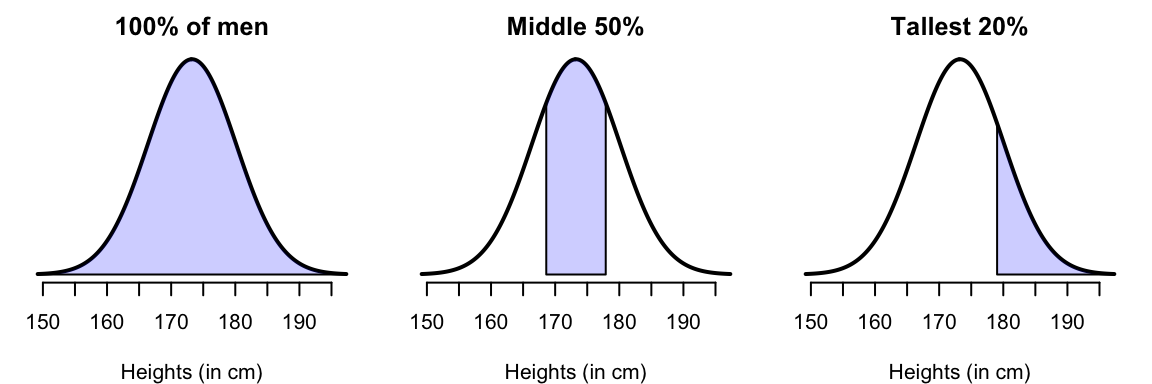
FIGURE 13.9: The heights of husbands, with certain percentages shaded
Importantly, for any normal distribution, whatever the mean or standard deviation, the areas under the smoothed curve approximately follow this important rule: The 68–95–99.7 rule.
Definition 13.11 (The 68–95–99.7 Rule (or the Empirical Rule)) For any bell-shaped distribution, approximately:
- 68% of observations lie within one standard deviation of the mean;
- 95% of observations lie within two standard deviations of the mean;
- 99.7% of observations lie within three standard deviations of the mean.
The animation below shows how the 68–95–99.7 works.
The 68–95–99.7 rule can be used to understand variables that have an approximate normal distribution. For example, consider the heights of husbands again (Fig. 13.10); the sample mean height is \(\bar{x} = 173.2\)cm; the sample standard deviation is \(s = 6.88\)cm. Using the 68–95–99.7 rule, approximately 68% of the husbands would have heights between
- \(173.2 - 6.88 = 166.3\)cm and
- \(173.2 + 6.88 = 180.1\)cm.
(In fact, 71% of husbands in the sample are between 166.3cm and 180.1cm tall, close to the expected 68%.) Similarly, approximately 95% of the husbands would have heights between
- \(173.2 - (2\times 6.88) = 159.4\)cm and
- \(173.2 + (2\times 6.88) = 187.0\)cm.
The empirical rule indicates that 99.7% of observations are within 3 standard deviations of the mean. That is, almost all observations are within three standard deviations of the mean.
This suggests a rule for identifying outliers in approximately bell-shaped distributions: any observation more than 3 standard deviations away from the mean is unusual, so may be considered an outlier. More generally, this rule is often applied to approximately symmetric distributions.
Bell-shaped (normal) distributions are studied further later (for example, Chap. 17).
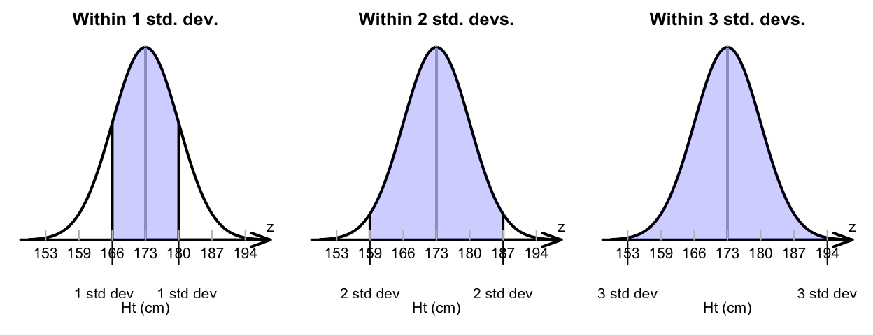
FIGURE 13.10: The heights of husbands, showing the 68–95–99.7 rule in use
13.5.2 The standard deviation rule for identifying outliers
One rule for identifying outliers is based on the 68–95–99.7 rule.
This rule uses the mean and the standard deviation, so this rule is suitable for approximately symmetric distributions (when means and standard deviations are sensible numerical summaries to use). Although this rule is based on normal distributions, it has proved useful for many approximately-symmetric distributions.
All rules for identifying outliers are arbitrary. For example, the standard deviation rule is sometimes given slightly differently; for example, outliers identified as observations more than 2.5 standard deviations away from the mean. Since all rules for identifying outliers are arbitrary, both rules are acceptable.
13.5.3 The IQR rule for identifying outliers
Since the standard deviation rule for identifying outliers relies on the mean and standard deviation, it is not appropriate for non-symmetric distributions. Another rule is needed for identifying outliers in these situations: the IQR rule.
Definition 13.13 (IQR rule for identifying outliers) The IQR rule identifies mild and extreme outliers as:
Extreme outliers: observations \(3\times \text{IQR}\) more unusual than \(Q_1\) or \(Q_3\).
Mild outliers: observations \(1.5\times \text{IQR}\) more unusual than \(Q_1\) or \(Q_3\) (that are not also extreme outliers).
This definition is much easier to understand using an example.
Example 13.10 (IQR rule for identifying outliers) An engineering project (Hald 1952) studied a new building material, to estimate the average permeability.
Measurements of permeability time (the time for water to permeate the sheets) were taken from 81 pieces of material (in seconds). For these data \(Q_1 = 24.7\) and \(Q_3 = 50.6\), so we find that \(\text{IQR} = {50.6 - 24.7 = 25.9}\). Then, extreme outliers observations are \(3\times 25.9 = 77.7\) more unusual than \(Q_1\) or \(Q_3\). That is, extreme outliers are observations:
- more unusual than \(24.7 - 77.7 = -53.0\) (that is, less than \(-53\)); or
- more unusual than \(50.6 + 77.7 = 128.3\) (that is, greater than \(128.3\)).
Mild outliers observations are \(1.5\times 25.9 = 38.9\) more unusual than \(Q_1\) or \(Q_3\) (that are not also extreme outliers). That is, mild outliers are
- more unusual than \(24.7 - 38.9 = -14.2\) (that is, less than \(-14.2\)); or
- more unusual than \(50.6 + 38.9 = 89.5\) (that is, greater than \(89.5\)).
You don’t need to do this (that’s what software is for), but you do need to understand what the software is doing. Construction of the boxplot is shown in the animation below.
13.5.4 When to use which rule?
In summary, two common ways to identify outliers are:
- For approximately symmetric distributions: use the standard deviation rule.
- For any distribution, but primarily for those skewed or with outliers: use the IQR rule.
But remember: All rules for identifying outliers are arbitrary!
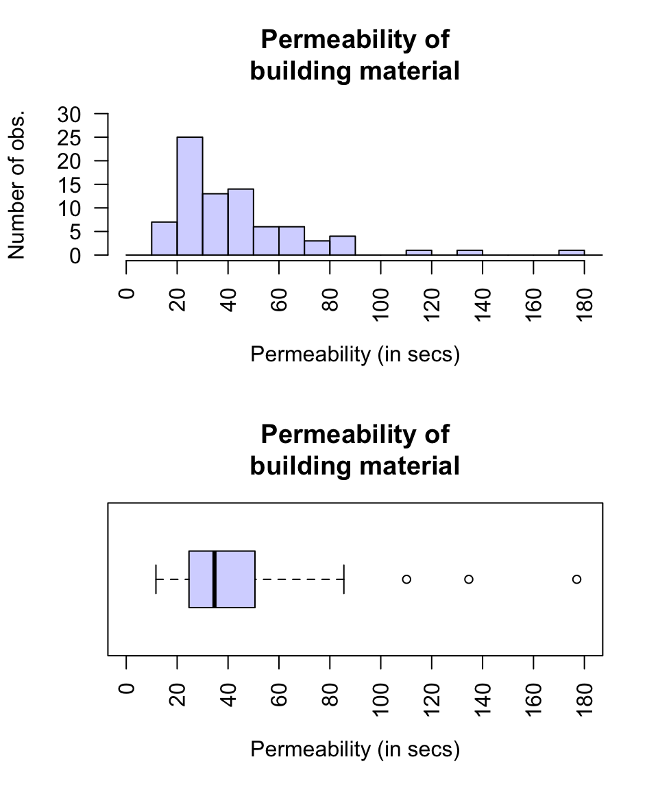
FIGURE 13.11: A boxplot and histogram for the permeability data
Think 13.10 (Understanding data summaries) In an American study (Tager et al. 1979), the lung capacity (FEV) of youth aged 3 to 19 was measured. The data are slightly skewed right, and the average FEV is about 2.6 litres, The FEV varies from about 0.8 to 5.8 litres, with no outliers.
Using this information, sketch the boxplot and the histogram for the data.