22.3 Confidence intervals: One mean
We don’t know the value of \(\mu\) (the paremeter), the population mean, but we have an estimate: the value of \(\bar{x}\), the sample mean (the statistic). The actual value of \(\mu\) might be a bit larger than \(\bar{x}\), or a bit smaller than \(\bar{x}\); that is, \(\mu\) is probably about \(\bar{x}\), give-or-take a bit.
Furthermore, we have seen that the values of \(\bar{x}\) vary from sample to sample (sampling variation), and noted that they vary with an approximate normal distribution. So, using the 68–95–99.7 rule, we could create an approximate 95% interval for the plausible values of \(\mu\) that may have given the observed values of the sample mean. This is a confidence interval.
A confidence interval (CI) for the population mean is an interval surrounding a sample mean. In general, an approximate 95% confidence interval (CI) for \(\mu\) is \(\bar{x}\) give-or-take about two standard errors. In general, the confidence interval (CI) for \(\mu\) is
\[ \bar{x} \pm \overbrace{(\text{Multiplier}\times\text{s.e.}(\bar{x}))}^{\text{Called the `margin of error'}}. \] For an approximate 95% CI, the multiplier is, as usual, about \(2\) (since about 95% of values are within two standard deviations of the mean from the 68–95–99.7 rule).
We often find 95% CIs, but we can find a CI with any level of confidence: we just need a different multiplier. We’ll just use a multiplier of \(2\) (and hence find approximate 95% CIs), and otherwise use software. Commonly, CIs are computed at 90%, 95% and 99% confidence levels.
If we collected many samples of a specific size, \(\bar{x}\) and \(s\) would be different for each sample, so the calculated CI would be different for each. Some CIs would straddle the population mean \(\mu\), and some would not; and we never know if the CI computed from our single sample straddles \(\mu\) or not.
Loosely speaking, there is a 95% chance that our 95% CI straddles \(\mu\). For a CI computed from a single sample, we don’t know if our CI includes the value of \(\mu\) or not. The CI could also be interpreted as the range of plausible values of \(\mu\) that could have produced the observed value of \(\bar{x}\).

Example 22.1 (School bags) A study of the school bags that 586 children (in Grades 6–8 in Tabriz, Iran) take to school found that the mean weight was \(\bar{x} = 2.8\) kg with a standard deviation of \(s=0.94\) kg (Dianat et al. 2014).
The parameter is the population mean weight of school bags for Iranian children in Grades 6–8.
Of course, another sample of 586 children would produce a different sample mean: the sample mean varies from sample to sample.
The standard error of the sample mean is
\[ \text{s.e.}(\bar{x}) = \frac{s}{\sqrt{n}} = \frac{0.94}{\sqrt{586}} = 0.03883; \] see Fig. 22.1. The approximate 95% CI for the population mean school-bag weight is
\[ 2.8\pm(2 \times 0.03883), \] or \(2.8\pm0.07766\). (The margin of error is 0.07766.) This is equivalent to an approximate 95% CI from 2.72 kg to 2.88 kg. This CI has a 95% chance of straddling the population mean bag weight.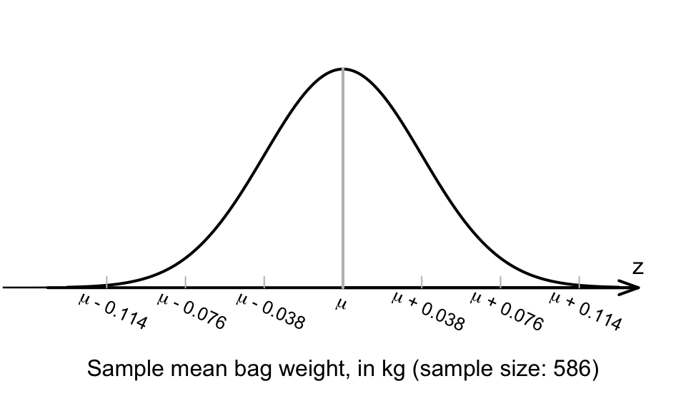
FIGURE 22.1: The normal distribution, showing how the sample mean bag weight varies in samples of size \(n=586\)
Example 22.2 (Black bears) A study of American black bears (Bartareau 2017) found that the mean weight of the \(n = 185\) male bears in their study was \(\bar{x} = 84.9\) kg, with a standard deviation of \(s = 51.1\) kg.
The parameter of interest is the population mean weight of an American black bear, \(\mu\).
Using the sample information, the standard error of the mean is
\[ \text{s.e.}(\bar{x}) = \frac{s}{\sqrt{n}} = \frac{51.1}{\sqrt{185}} = 3.756947, \] so the approximate 95% CI is from \[ 84.9 - (2 \times 3.756947) = 77.38611 \] to \[ 84.9 + (2 \times 3.756947) = 92.41389. \] The approximate 95% CI is from 77.4 to 92.4 kg. We would say:
The article gives the exact CI as 77.4 to 99.5 kg, agreeing with the CI we calculated.We are approximately 95% confidence that the population mean weight of male American black bears is between 77.4 and 92.4 kg.