35.7 Confidence intervals
Reporting the CI for the slope is also useful, which can be obtained from software or computed manually.
CIs have the form \[ \text{statistic} \pm ( \text{multiplier} \times \text{standard error}), \] The multiplier is two for an approximate 95% CI, so (using the standard error reported by the software), we obtain \(-0.181 \pm (2\times 0.029)\), or \(-0.181 \pm 0.058\), or from \(-0.239\) to \(-0.123\).
Software can be asked to produce exact CIs too (jamovi: Fig. 35.11; SPSS: Fig. 35.12). The approximate and exact 95% CIs are very similar.
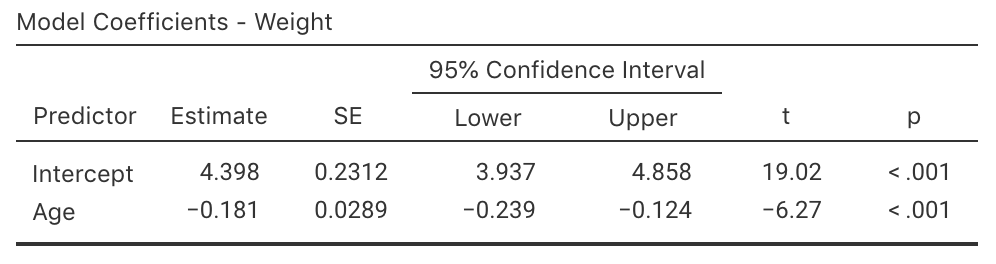
FIGURE 35.11: jamovi output for the red-deer data, including the CIs
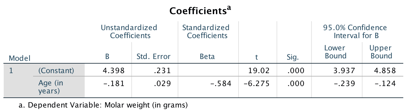
FIGURE 35.12: SPSS output for the red-deer data, including the CIs
We write:
The sample presents very strong evidence (\(P < 0.001\); \(t = -6.275\)) of a relationship between age and the weight of molars in male red deer (slope: \(-0.181\); \(n= 78\); 95% CI from \(-0.239\) to \(-0.124\)) in the population.
Example 35.5 (Emergency department patients) In Example 35.4, the jamovi output does not give the 95% CI for the slope.
However, since CIs have the form
\[
\text{statistic} \pm ( \text{multiplier} \times \text{standard error}),
\]
the CI is easily computed:
\[
-0.34790 \pm (2\times 0.046672),
\]
or \(-0.34790 \pm 0.093344\).
This is equivalent to \(-0.441\) to \(-0.255\).
Combining with information from Example 35.4, we write:
The sample presents very strong evidence (\(P < 0.001\); \(t = -7.45\)) of a relationship between the mean number of ED patients and the numbers of days after welfare distribution (slope: \(-0.348\); \(n = 30\); 95% CI from \(-0.441\) to \(-0.255\)) in the population.