34.1 Correlation coefficients

Describing the linear relationship between two quantitative variables, requires a description of the form, direction and variation. A correlation coefficient is a single number encapsulating all this information.

In the population, the unknown value of the correlation coefficient is denoted \(\rho\) (‘rho’); in the sample the value of the correlation coefficient is denoted \(r\). As usual, \(r\) (the statistic) is an estimate of \(\rho\) (the parameter), and the value of \(r\) is likely to be different in every sample (that is, sampling variation exists).

The symbol \(\rho\) is the Greek letter ‘rho,’ pronounced ‘row,’ as in ‘row your boat’.

Correlation coefficients only apply if the form is approximately linear, so checking if the relationship is linear first (using a scatterplot) is important. Here, the Pearson correlation coefficient is discussed, which is suitable for describing linear relationships between quantitative data¹⁵.

The Pearson correlation coefficient only make sense if the relationship is approximately linear.

The values of \(\rho\) and \(r\) are always between \(-1\) and \(+1\). The sign indicates whether the relationship has a positive or negative linear association, and the value of the correlation coefficient tells us the strength of the relationship:

\(r=0\) means no linear relationship between the two variables: Knowing how the value of \(x\) changes tells us nothing about how the value of \(y\) changes.
\(r=+1\) means a perfect, positive relationship: knowing the value of \(x\) means we can perfectly predict the value of \(y\) (and larger values of \(y\) are associated with larger values of \(x\), in general).
\(r=-1\) means a perfect, negative relationship: knowing the value of \(x\) means we can perfectly predict the value of \(y\) (and larger values of \(y\) are associated with smaller values of \(x\), in general).

The animation below demonstrates how the values of the correlation coefficient work.

Numerous example scatterplots were shown in Sect. 33.3; a correlation coefficient is not relevant for Plots C, D, E or H, as those relationships are not linear. In Plot A, the correlation coefficient will be positive, and reasonably close to one. In Plot B, the correlation coefficient will be negative, but not that close to \(-1\). In Plot F, the correlation coefficient will close to zero.

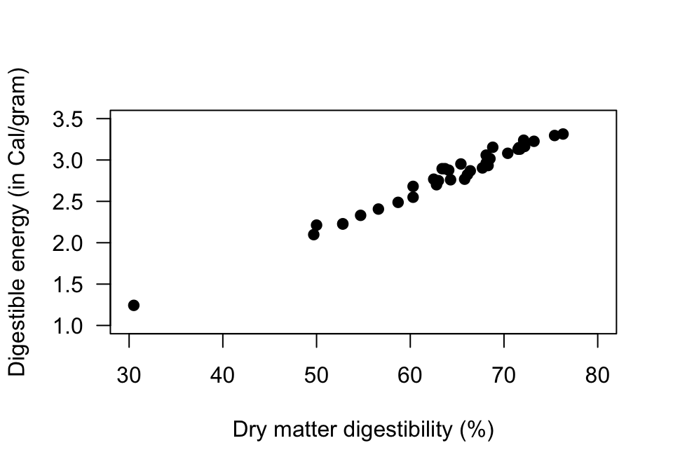
Example 34.1 (Correlation coefficients) For the red deer data (Fig. 33.2), \(r = -0.584\). The value of \(r\) is negative, because, in general, older deer (\(x\)) are associated with smaller weight molars (\(y\)).

FIGURE 34.1: Scatterplot for the sheep-food data

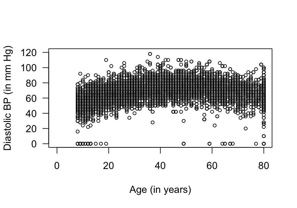
Example 34.2 (Correlation coefficients) Consider the plot in Fig. 34.2 from the NHANES data. This scatterplot of diastolic BP against age is not linear, so a correlation coefficient is not appropriate.

FIGURE 34.2: A scatterplot of the diastolic blood pressure against age for the NHANES data

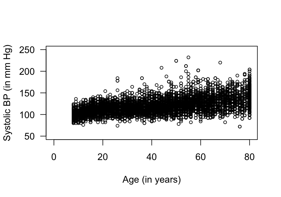
Example 34.3 (Correlation coefficients) Consider the plot in Fig. 34.3 from the NHANES data. This scatterplot of systolic BP against age is approximately linear, so a correlation coefficient is appropriate. The correlation coefficient is \(r = 0.532\).

FIGURE 34.3: A scatterplot of the systolic blood pressure against age for the NHANES data

Think 34.1 (Estimate \(r\)) A study evaluated various food mixtures for sheep (Moir 1961). One combination of variables that was assessed is shown in Fig. 34.1.

Estimate the value of \(r\).

\(r\) will be a positive number (since the scatterplot shows a positive linear relationship), and its value will be close to 1 as the relationship looks very strong.

Think 34.2 (Guess the value of \(r\)) Earlier, we looked at the NHANES data to explore the relationship between direct HDL cholesterol and current smoking status. The NHANES project is an observational study, so confounding is a potential issue. For this reason, relationships between the response and extraneous variables, and between explanatory and extraneous variables, should be examined.

For example, the relationship between Age (an extraneous variables) and direct HDL cholesterol (the response variable) is shown in Fig. 34.4.

How would you describe the relationship? What do you guess for the value of \(r\)?

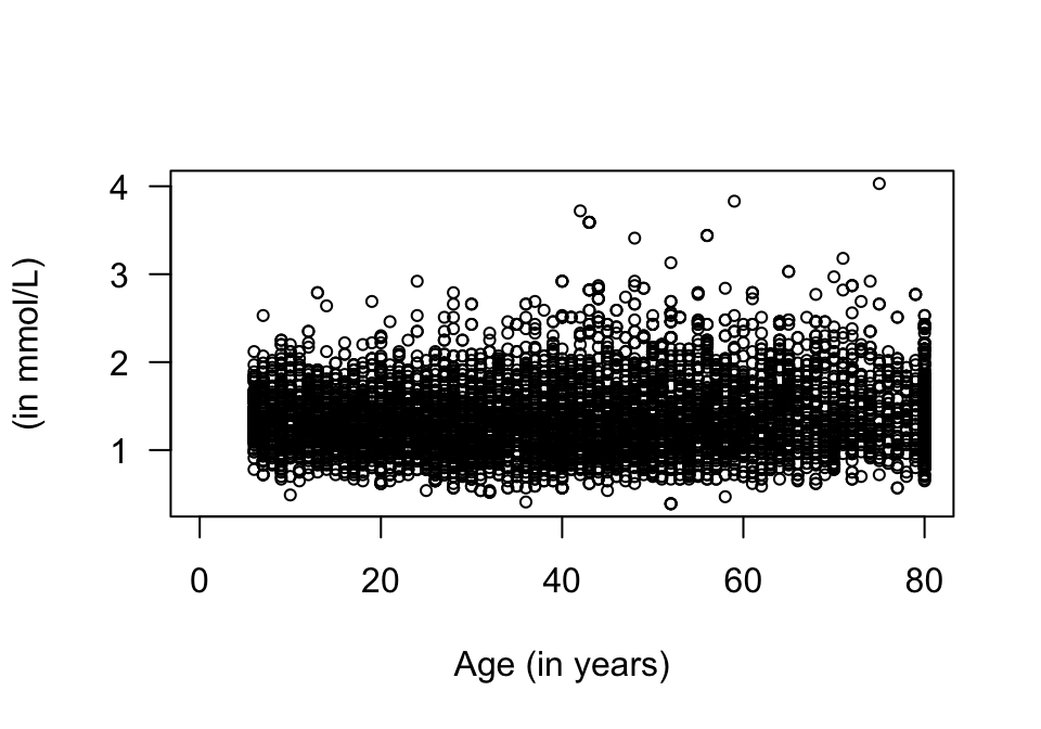
FIGURE 34.4: Direct HDL cholesterol plotted against age for the NHANES data

Not much relationship: the mean of the direct HDL cholesterol concentration is similar for any age. Perhaps describe the scatterplot as ‘little relationship.’ We cannot make good guess about the value of \(r\), but it will be near zero.

The web page http://guessthecorrelation.com makes a game out of trying to guess the correlation coefficient!

References

Moir RJ. A note on the relationship between the digestible dry matter and the digestable energy content of ruminant diets. Australian Journal of Experimental Agriculture and Animal Husbandry. 1961;1:24–6.

Other types of correlation coefficients also exist, such as the Spearman correlation, which may be used for monotonic, non-linear relationships.↩︎