27.5 \(P\)-values: One mean
This is the decision-making progress so far:
- Assume that the population mean is \(37.0^\circ\text{C}\) (this is \(H_0\)).
- Based on this assumption, describe what to expect from the sample means (Fig. 27.2).
- The observed statistic is computed, relative to what is expected using a \(t\)-score (Fig. 27.3): \(t=-5.453\).
The value of the \(t\)-score shows that the value of \(\bar{x}\) is highly unusual. How unusual can be assessed more precisely using a \(P\)-value, which is used widely in scientific research. The \(P\)-value is a way of measuring how unusual an observation is (if \(H_0\) is true).
\(P\) values can be approximated using the 68–95–99.7 rule and a diagram (Sect. 27.5.1), but more commonly by using software (Sect. 27.5.2).
27.5.1 Approximating \(P\)-values using the 68–95–99.7 rule
The \(P\)-value is the area more extreme than the calculated \(t\)-score. For example:
If the calculated \(t\)-score was \(t=-1\), the two-tailed \(P\)-value would be the shaded area in Fig. 27.4 (top panel): About 32%, based on the 68–95–99.7 rule. Because the alternative hypothesis is two-tailed, both sides of the mean are considered: the \(P\)-value would be the same if \(t=+1\).
If the calculated \(t\)-score was \(t=-2\), the two-tailed \(P\)-value would be the shaded area shown in Fig. 27.4 (bottom panel): About 5%, based on the 68–95–99.7 rule. Because the alternative hypothesis is two-tailed, both sides of the mean are considered: the \(P\)-value would be the same if \(t=+2\).
Clearly, from what the \(P\)-value means, a \(P\)-value is always between 0 and 1.
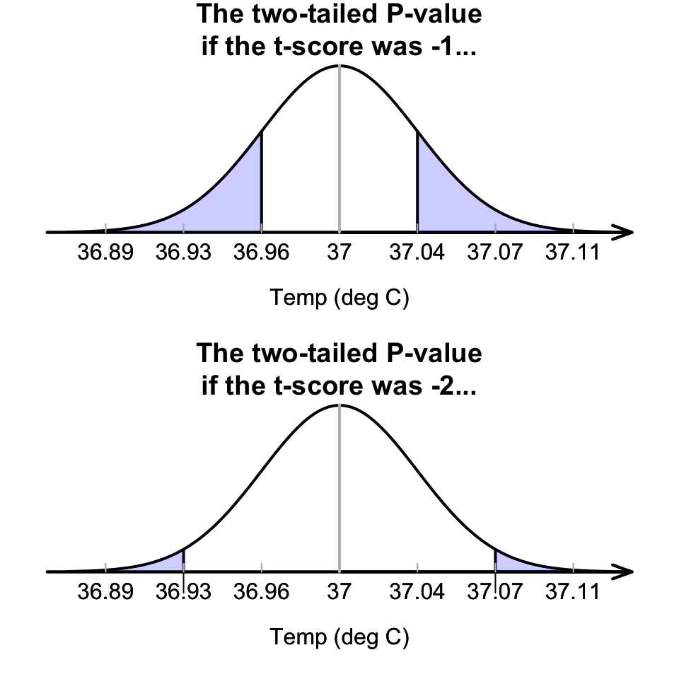
FIGURE 27.4: Computing \(P\)-values for the body temperature data
27.5.2 Finding \(P\)-values using sofware
Software computes the
\(t\)-score and a precise \(P\)-value
(jamovi: Fig. 27.5;
SPSS: Fig. 27.6).
The output
(in jamovi, under the heading p;
in SPSS, under the heading Sig. (2-tailed))
shows that the \(P\)-value is indeed very small.
Although SPSS reports the \(P\)-value as 0.000,
\(P\)-values can never be exactly zero,
so we interpret this as
‘zero to three decimal places,’
or that \(P\) is less than 0.001
(written as \(P<0.001\), as jamovi reports).
0.000,
it really means (and we should write) \(P<0.001\):
That is, the \(P\)-value is smaller than 0.001.
This \(P\)-value means that, assumpting \(\mu=37.0^\circ\)C, observing a sample mean as low as \(36.8051^\circ\)C just through sampling variation (from a sample size of \(n=130\)) is almost impossible. And yet, we did…
Using the decision-making process, this implies that the initial assumption (the null hypothesis) is contradicted by the data: The evidence suggests that the population mean body temperature is not \(37.0^\circ\text{C}\).
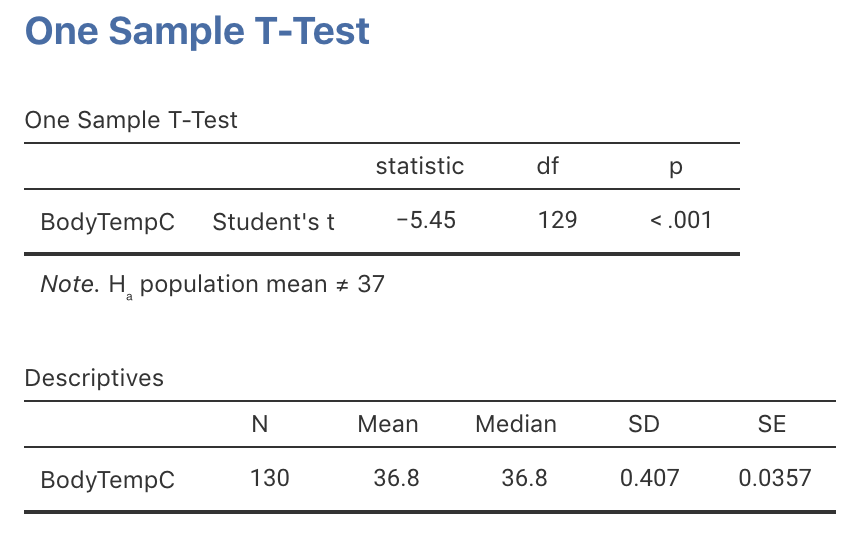
FIGURE 27.5: jamovi output for conducting the \(t\)-test for the body temperature data
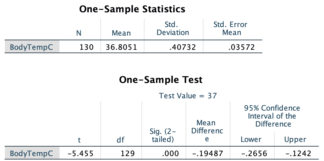
FIGURE 27.6: SPSS output for conducting the \(t\)-test for the body temperature data
SPSS always produces two-tailed \(P\)-values,
calls then Significance values,
and labels them as Sig.