D.5 Defining and using custom colors
We need to distinguish between defining individual colors, converting colors, and defining color palettes. And once we defined new color palettes, we need to know how we can use them in creating visualizations (in both base R and the ggplot2 package).
D.5.1 Defining colors
As there are many different ways to describe a color, there are many different ways to define a color. Here, we will only discuss three common ways of defining a color in R:
- by color name (e.g.,
col = c("black", "white"))
See colors() for the list of 657 color names available in base R — and note that every color is represented in character type.
- by HEX (hexadecimal) code (e.g.,
col = c("#000000", "#FFFFFF"))
Such HEX codes essentially specify a triplet of RGB values in hexadecimal notation. The three bytes represent a color’s red, green and blue components by a number in the range from 00 to FF (in hexadecimal notation), corresponding to a range from 0 to 255 (in decimal notation). As this way of representing color is popular online (in HTML), they are also known as web colors.
Note that, in R, each HEX code is represented in character type, with the hash tag # as a prefix.
HEX codes with more than six digits following the # symbol encode opacity information (in the last two digits), but this information is often lost in color conversions.
- by RGB (red-green-blue) values (e.g.,
col = c(rgb(red = 0, green = 0, blue = 0, maxColorValue = 255), rgb(255, 255, 255, maxColorValue = 255)))
Such RGB values are more traditional and can be entered and converted in most computer systems.
In R, we can use the rgb() function to enter the red, green, and blue value of a color, as well as an optional opacity (or transparency) value alpha. Note that we need to specify the maxColorValue = 255 to scale these values in the most common fashion (from 0 to 255).
If it seems confusing that the same color can be defined in several ways, consider the fact that the symbols “2,” “two,” “zwei,” “II” and “10 in binary notation” all denote the same number. If a simple number can be represented in so many ways, its less surprising that a complex phenomenon like color can be expressed in multiple representations.
Importantly, the vast majority of colors can be expressed in any system and can thus be translated from one system into another (though some features, like color opacity, may get lost in translation). The following example shows how a vector of colors can be defined in multiple ways.
Defining colors in different ways
For instance, the following graph shows the visual representation, color name, HEX codes, and RGB values of a vector my_cols that describes four distinct colors:
my_cols <- c("black", "orange", "olivedrab3", "steelblue")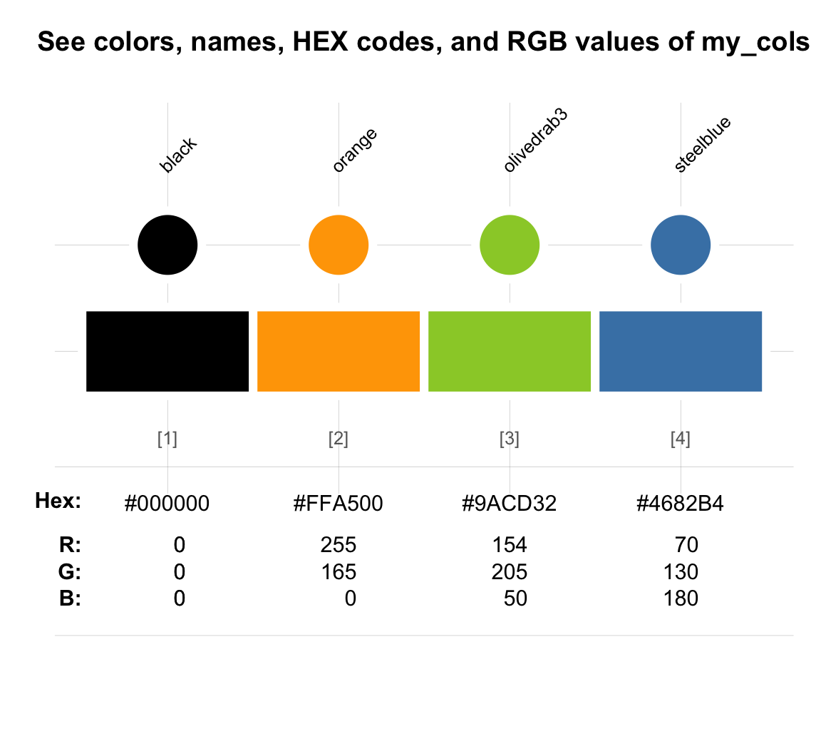
The three ways of expressing each individual color shown are interchangeable.
In the graph above, we can see that the color palette my_cols could have been defined in the following ways:
p1 <- c("black", "orange", "olivedrab3", "steelblue")  # 1. R color names

p2 <- c("#000000", "#FFA500", "#9ACD32", "#4682B4")    # 2. HEX codes

p3 <- c(rgb(  0,   0,   0, maxColorValue = 255),       # 3. RGB values
        rgb(255, 165,   0, maxColorValue = 255),
        rgb(154, 205,  50, maxColorValue = 255),
        rgb( 70, 130, 180, maxColorValue = 255))

p4 <- c("black", "orange",                             # 4. R color names,
        "#9ACD32",                                     #    HEX codes, and
        rgb( 70, 130, 180, maxColorValue = 255))       #    RGB values
Note that both color names and HEX codes were entered within quotation marks (i.e., yield vectors of type character). Inspecting the resulting vectors shows the following:
# Inspect resulting vectors:
p1
#> [1] "black"      "orange"     "olivedrab3" "steelblue"
p2
#> [1] "#000000" "#FFA500" "#9ACD32" "#4682B4"
p3
#> [1] "#000000" "#FFA500" "#9ACD32" "#4682B4"
p4
#> [1] "black"   "orange"  "#9ACD32" "#4682B4"

# Check equality:
all.equal(p1, p2)
#> [1] "4 string mismatches"
all.equal(p2, p3)
#> [1] TRUE
all.equal(p1, p4)
#> [1] "2 string mismatches"
Thus, the R color names and HEX codes (entered as character objects) remain unchanged.
Consequently, evaluating all.equal(p1, p2) tells us that they are totally different (i.e., “4 string mismatches.”)
By contrast, entering the rgb() values of p3 converted the RGB values into HEX values (as character objects).
Thus, p2 and p3 are identical character vectors, and each vector of p1–p3 differs from p4 by exactly two elements.
But what about our goal of defining the same color vectors? Have we failed because the resulting vectors show some differences? Well, the answer depends on what we mean by “the same.” Despite using different representations, all four vectors describe the same colors, as the following comparison graph reveals:
seecol(list(p1, p2, p3, p4),
       col_brd = "white", lwd_brd = 4,
       pal_names = c("p1 (names)", "p2 (HEX)", "p3 (RGB)", "p4 (mix)"),
       title = "Defining the same colors in 4 ways")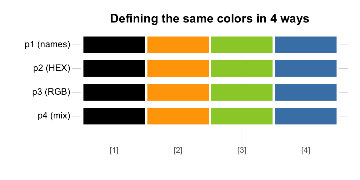
Same different colors
A rose may be a rose (see ds4psy::flowery), but “red” isn’t “red2” (see seecol(grepal("^red"))).
So what if we had chosen slightly different RGB values to define our colors?
To test this, we can define a color vector p3b in which each value deviates by 1 from the previous RGB values:
p3b <- c(rgb(  1,   1,   1, maxColorValue = 255),       # 3. RGB values
         rgb(254, 166,   1, maxColorValue = 255),
         rgb(155, 206,  51, maxColorValue = 255),
         rgb( 71, 131, 181, maxColorValue = 255))

seecol(list(p3, p3b),
       col_brd = "white", lwd_brd = 4,
       pal_names = c("p3 (RGB)", "p3b (RGB+1)"),
       title = "See a difference?")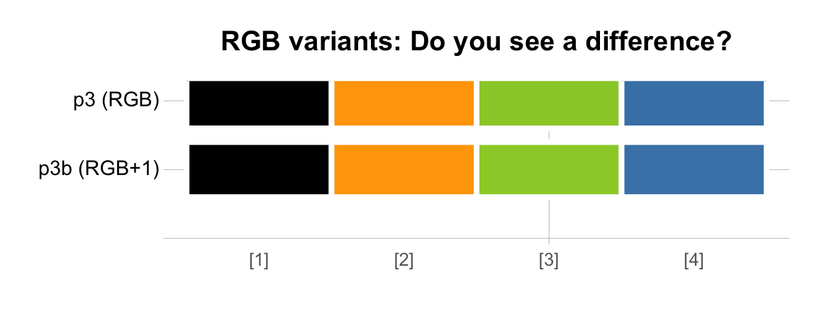
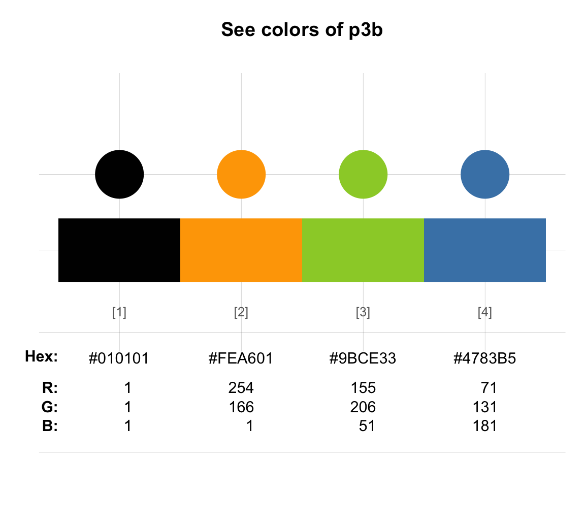
Thus, colors with similar RGB values are perceptually fairly similar. However, colors that may essentially look the same are still different for some purposes, just like it may or may not make a difference whether the price of some product is $4.99 or $5.00. For instance, the following comparison shows that using slightly different RGB values implies that R no longer recognizes the original colors’ names and encodes the new colors with slightly different HEX codes:
The option of defining colors in different ways is both a benefit and a burden for designers: It adds flexibility, but comes at the cost of familiarizing ourselves with multiple systems and corresponding tools. On the bright side, most R users do not need to worry about all this, as long as they can remember the names of their preferred colors or some functions for specifying and manipulating color palettes.
Other color systems
Knowing that colors can be described by their names, HEX codes, and RGB values is perfectly sufficient for most R users. Nevertheless, there are many additional ways for defining and expressing colors (see Wikipedia: Color model). In R, colors are sometimes specified by their HSV (hue-saturation-value) or HCL (hue-chroma-luminance) values.
The HSV (hue-saturation-value) system is a simple transformation of the RGB color space and is used in many software systems (see
?hsvfor corresponding R functions).In the HCL system, the hue specifies a color type, chroma the color’s colorfulness, and luminance its brightness (see
?hclfor details).
According to Zeileis et al. (2020), the HCL system is more systematic than the HSV system and more suitable for capturing human color perception.
Since R version 3.6.0 (released in April 2019), some default colors of R have been changed to use the HCL system (see the hcl.colors() function of grDevices for details and available color palettes).
D.5.1.1 Converting colors
R also comes with powerful color conversion functions that allow translating color values between the different systems.
For instance, we can use the col2rgb() function of grDevices to obtain the RGB values that correspond to specific R color names.
As col2rgb() requires a matrix-like object (rather than a vector) as its input to its col argument, we use the newpal() function of unikn with as_df = TRUE to define a color palette my_pal as a data frame:
library(unikn)

# Define a vector with colors:
col_names <- c("black", "grey", "white", "firebrick", "forestgreen", "gold", "steelblue")

# Define corresponding color palette:
my_pal <- newpal(col = col_names, names = col_names, as_df = TRUE)

# Verify data structure:
is.vector(my_pal)
#> [1] FALSE
is.data.frame(my_pal)
#> [1] TRUE

# See colors (and details):
seecol(my_pal,
       col_brd = "black", lwd_brd = 2,
title = "See the colors, HEX codes, and RGB values of my_pal") 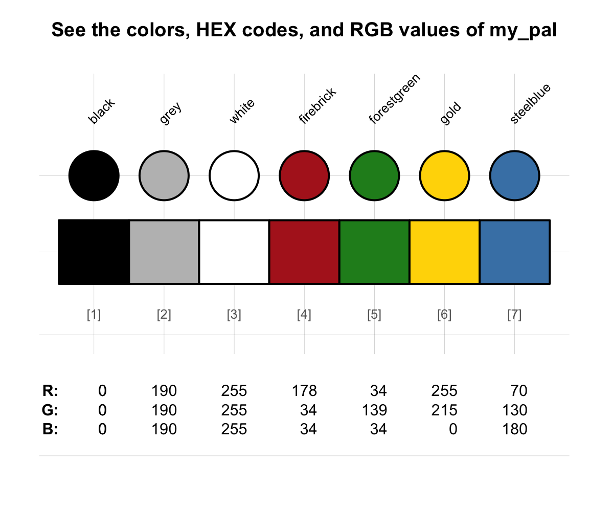
To obtain the RGB values of my_pal, we can either use the col2rgb() function (to obtain a matrix of RGB values) or the seecol() function of unikn (for visual inspection):
col2rgb(my_pal)
#>       black grey white firebrick forestgreen gold steelblue
#> red       0  190   255       178          34  255        70
#> green     0  190   255        34         139  215       130
#> blue      0  190   255        34          34    0       180
When frequently needing to convert colors between different color spaces, consider using the colorspace package (Ihaka et al., 2020), which defines color-class objects that can be converted into a variety of color spaces (including RGB, sRGB, HSV, HLS, XYZ, LUV, LAB, polarLUV, and polarLAB).
D.5.2 Defining color palettes
In Section D.2.1, we distinguished between individual colors and color palettes, which are sets of colors to be used together. Defining our own color palettes is a great way to maintain a consistent color scheme for multiple graphs in a report or thesis.
It is easy to define our own color palettes. More precisely, it only is easy to combine existing colors to define a new color palette. Whether the new color palette will work well for your current purposes is a different matter (and it often makes sense to let expert designers do the work when creating new color schemes).
Corresponding to the three common ways of defining a color in R, we can define new color palettes in (at least) three ways.
To illustrate them, we will use some color-related functions provided by the unikn package. (Simply combining colors into vectors is often sufficient, but the newpal() function automatically returns our palettes as data frames with color names. The seecol() function allows inspecting the results of our definitions.)
- Starting from R color names:
pal_flag_de <- newpal(col = c("black", "red3", "gold"),
                      names = c("Schwarz", "Rot", "Gold"))

seecol(pal_flag_de,
       col_brd = "white", lwd_brd = 4,
       title = "Colors of the German flag",
       mar_note = "Approximation (based on R color names)")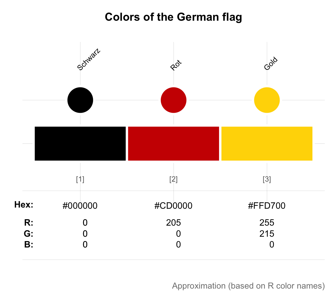
A good question to ask here is:
- How do we know the names of these colors?
In the current case, we knew that “black” denotes black and had a pretty good idea of what the result should look like.
Importantly, knowing that the other colors should show some form of “red” and “gold,” we searched for suitable shade by using the grepal() function of the unikn package (e.g., seecol(grepal("^red")), see Section D.4.3).
This way of “searching colors by name” worked fine here, but could not possibly find other available shades of red that go by different names (e.g., “coral,” “firebrick,” or “tomato”).
- Starting from HEX values:
# (a) Google logo colors:
# Source: https://www.schemecolor.com/google-logo-colors.php
color_google <- c("#4285f4", "#34a853", "#fbbc05", "#ea4335")
names_google <- c("blueberry", "sea green", "selective yellow", "cinnabar")
pal_google   <- newpal(color_google, names_google)
seecol(pal_google, col_brd = "white", lwd_brd = 6,
       title = "Colors of the Google logo",
       mar_note = "Source: <https://www.schemecolor.com/google-logo-colors.php>")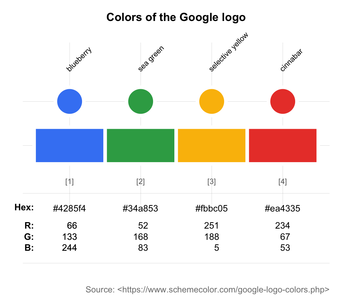
As most people do not memorize the HEX codes of colors, these values typically stem from color picking apps or technical manuals or sites that provide color definitions (see Section D.7.4 for links to online resources).
- Starting from RGB values, we can implement the Color Universal Design (CUD) recommendations of https://jfly.uni-koeln.de/color/ (see Figure 16 of Okabe & Ito, 2008):
# Barrier-free color palette
# Source: Okabe & Ito (2008): Color Universal Design (CUD):
#         Fig. 16 of <https://jfly.uni-koeln.de/color/>:

# (a) Vector of colors (as RGB values):
o_i_colors <- c(rgb(  0,   0,   0, maxColorValue = 255),  # black
                rgb(230, 159,   0, maxColorValue = 255),  # orange
                rgb( 86, 180, 233, maxColorValue = 255),  # skyblue
                rgb(  0, 158, 115, maxColorValue = 255),  # green
                rgb(240, 228,  66, maxColorValue = 255),  # yellow
                rgb(  0, 114, 178, maxColorValue = 255),  # blue
                rgb(213,  94,   0, maxColorValue = 255),  # vermillion
                rgb(204, 121, 167, maxColorValue = 255)   # purple
)

# (b) Vector of color names:
o_i_names <- c("black", "orange", "skyblue", "green", "yellow", "blue", "vermillion", "purple")

# (c) Use newpal() to combine colors and names:
pal_okabe_ito <- newpal(col = o_i_colors,
                        names = o_i_names)

# See palette:
seecol(pal_okabe_ito,
       title = "Color-blind friendly color palette",
       mar_note = "Source: Figure 16 of Okabe & Ito (2008); see <https://jfly.uni-koeln.de/color/>")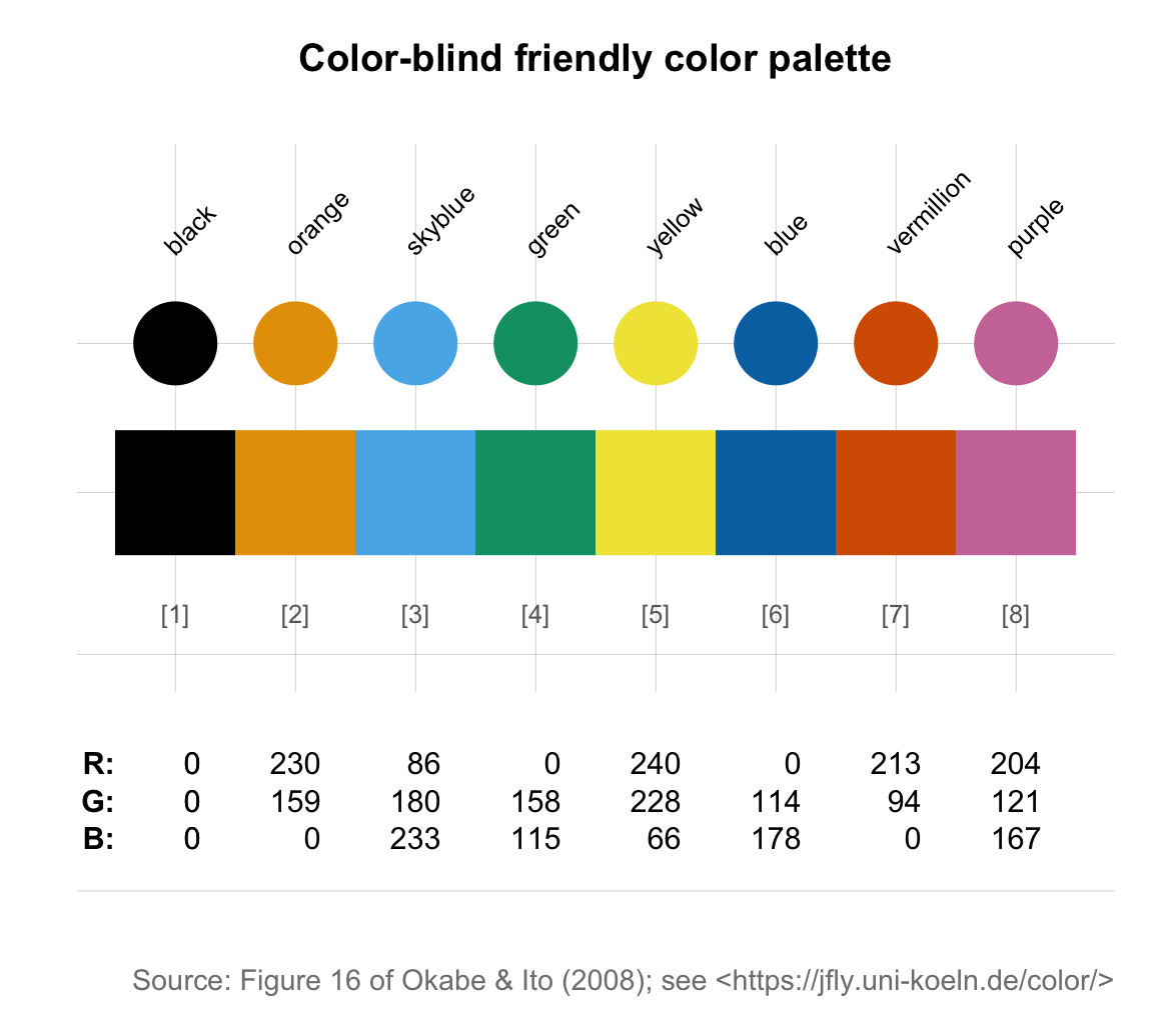
Again, the RGB values used for such definitions typically stem from color picking apps or technical manuals (see Section D.7.4 for links to online resources).
By creating a list of our new color palettes, we can print and compare them using the seecol() function:
# Compare custom color palettes:
my_pals <- list(pal_flag_de, pal_google, pal_okabe_ito)
seecol(my_pals, col_brd = "white", lwd_brd = 6,
       title = "Comparing custom color palettes")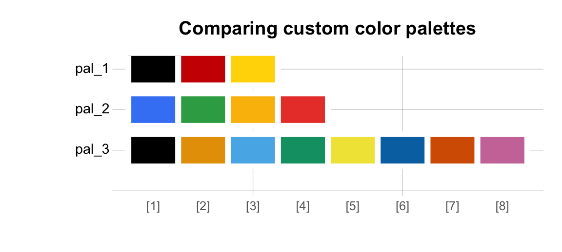
Both the seecol() and the usecol() functions also allow specifying an argument n for extending color palettes:
seecol(pal_flag_de, n = 5,
       col_brd = "white", lwd_brd = 5,
       title = "Extending custom color palette pal_de_flag (n = 5)")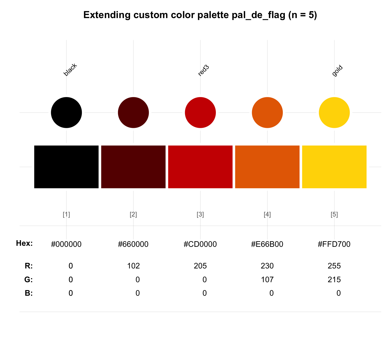
or modifying color palettes further (e.g., by adding transparency values alpha):
seecol(my_pals, n = 10, alpha = .50,
       col_brd = "white", lwd_brd = 8,
       pal_names = c("pal_flag_de", "pal_google", "pal_okabe_ito"),
       title = "Comparing custom palettes (with transparency)")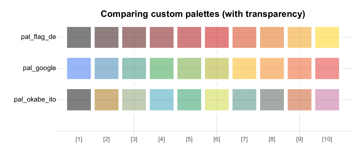
Practice
Define and compare the flags colors of France and the U.S.A.:
- look up their color definitions (e.g., at https://en.wikipedia.org/ or https://www.schemecolor.com);
- create corresponding color palettes (with appropriate color names);
- create a visualization that shows each flag’s colors.
Solution
The following solutions illustrate the difference between the U.S. and France, as far as their flag’s color palettes are concerned:
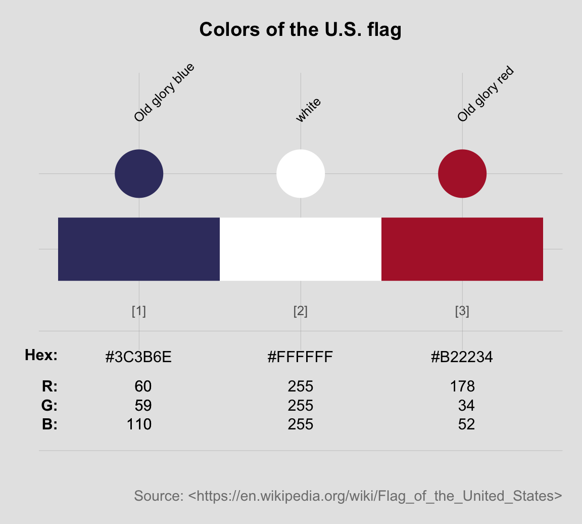
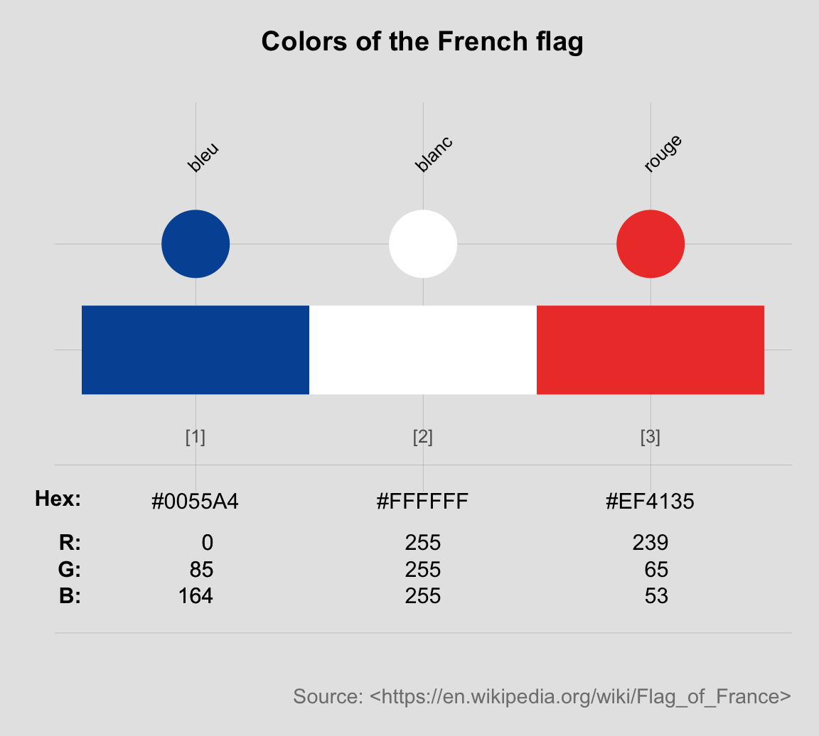
Beware: Please note that looking up colors can be a sensitive and controversial act, and we should always be careful in choosing and crediting our sources. For instance, Wikipedia notes at least three different definitions for the blue and red colors of the U.S. flag. Similarly, the specifications of the Tricolore colors at Wikipedia and Schemecolor.com agree in their HEX codes, but the latter states that the blue color of the French flag is called “USAFA blue.” I wonder whether French readers would agree? (Lots of material for conspiracy theories here…)
D.5.3 Using custom colors in base R
In Section D.3.6 we described how R’s default palette() can be set to a different color palette.
This is a quite radical step, as it changes all subsequent uses of palette().
A more common and less invasive way of using a particular color palette is by providing it as an argument to a plotting function.
Different color resources provide colors in different ways.
Color palettes are either defined as functions that return an output vector, data frame, or matrix,
or as R objects that are vectors, data frames, or matrices.
In many cases, just providing a vector of R color names works fine. However, some packages provide color palettes as data frames or functions with variable output types. As a uniform interface for using and modifying color palettes from various sources, the unikn package (Neth & Gradwohl, 2021) provides the usecol() function. Here are some examples of defining color palettes on the fly:
# Define 3 new palettes (from different sources):
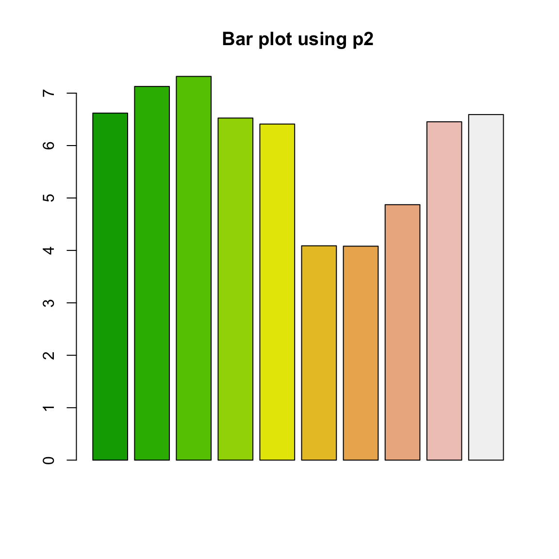
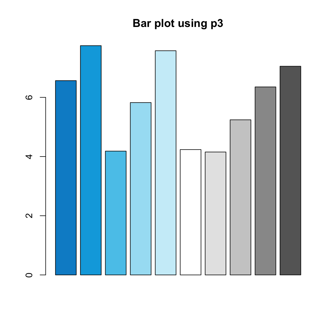
p1 <- usecol(c("orange", "olivedrab3", "steelblue")) # from R color names
p2 <- usecol(terrain.colors(10)) # from a color function
p3 <- usecol(pal_unikn) # from a color palette (as df)
# Example plots:
pie(rep(1, 8), col = p1, main = "Pie plot using p1")
barplot(runif(10, 4, 8), col = p2, main = "Bar plot using p2")
barplot(runif(10, 4, 8), col = p3, main = "Bar plot using p3")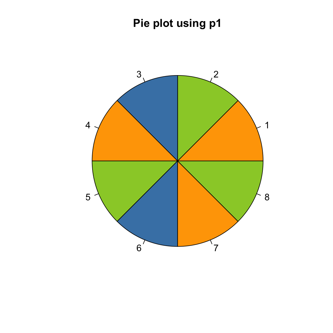
The usecol() function also allows mixing combinations of colors and color palettes, squeezing or stretching them to arbitrary lengths, and setting their transparency:
# Mixing a new color palette:
p1 <- usecol(pal = c(rev(pal_seeblau), "white", pal_pinky))

# Mixing, extending a color palette (and adding transparency):
p2 <- usecol(pal = c(rev(pal_seegruen), "white", pal_bordeaux), n = 15, alpha = .60)

# Defining and using a custom color palette:
p3 <- usecol(c("#E77500", "white", "black"), n = 7)

# Show set of color palettes:
seecol(list(p1, p2, p3), col_brd = "white", lwd_brd = 2,
       title = "Using usecol() to mix and modify color palettes")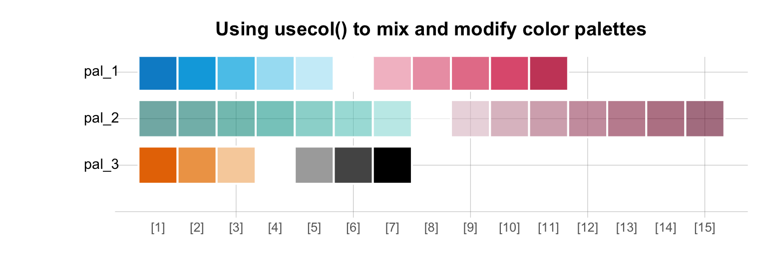
The basic idea of the usecol() and seecol() functions of the unikn package is that they provide an easy way of mixing and merging a variety of colors, color palettes, and color packages, without worrying about the details.
D.5.4 Using custom colors in ggplot2
- To use a particular base R color in a
ggplot()command, we can pass its name (as a character string) to functions that includes acolorargument:
library(ggplot2)
library(unikn)

# Choose a color (plus transparency):
my_col <- usecol(Pinky, alpha = 1/2)

# Using an individual color (as an argument):
ggplot(mpg) +
  geom_point(aes(x = displ, y = hwy),
             color = my_col, size = 4) +
  labs(title = "Using a custom color in ggplot2") +
  theme_classic()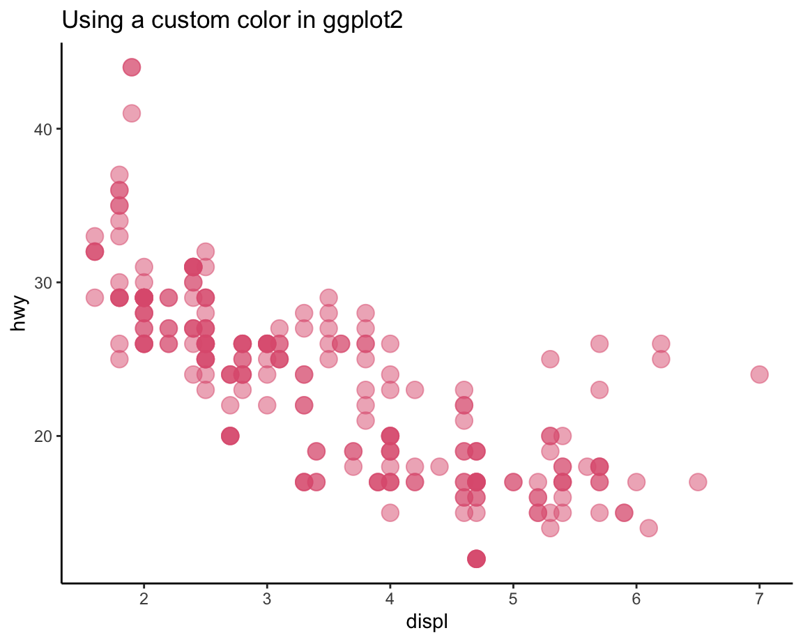
Note that placing the color = "steelblue" specification outside of the aes() function changed all points of our plot to this particular color.
- To define and use a new color palette
my_colorsin aggplot()command, we need to add thescale_color_manual()function that instructs ggplot to use a custom color scale for the current plot. Note thatscale_color_manual()expects to receive colorvalues, rather than mere color names, and a vector, rather than a data frame:
# Define color vector (in 4 different ways, see p4 above):
my_pal <- c("black", "orange",                         # R color names,
            "#9ACD32",                                 # HEX codes, and
            rgb( 70, 130, 180, maxColorValue = 255))   # RGB values

# Inspect colors:
my_pal
#> [1] "black"   "orange"  "#9ACD32" "#4682B4"
# seecol(my_pal)  # (see above)

# Use color palette (in ggplot):
ggplot(mpg) +
  geom_point(aes(x = displ, y = hwy, color = factor(cyl)), size = 4, alpha = .5) +
  scale_color_manual(values = my_pal) +
  labs(title = "Using a custom color palette in ggplot2") +
  theme_classic()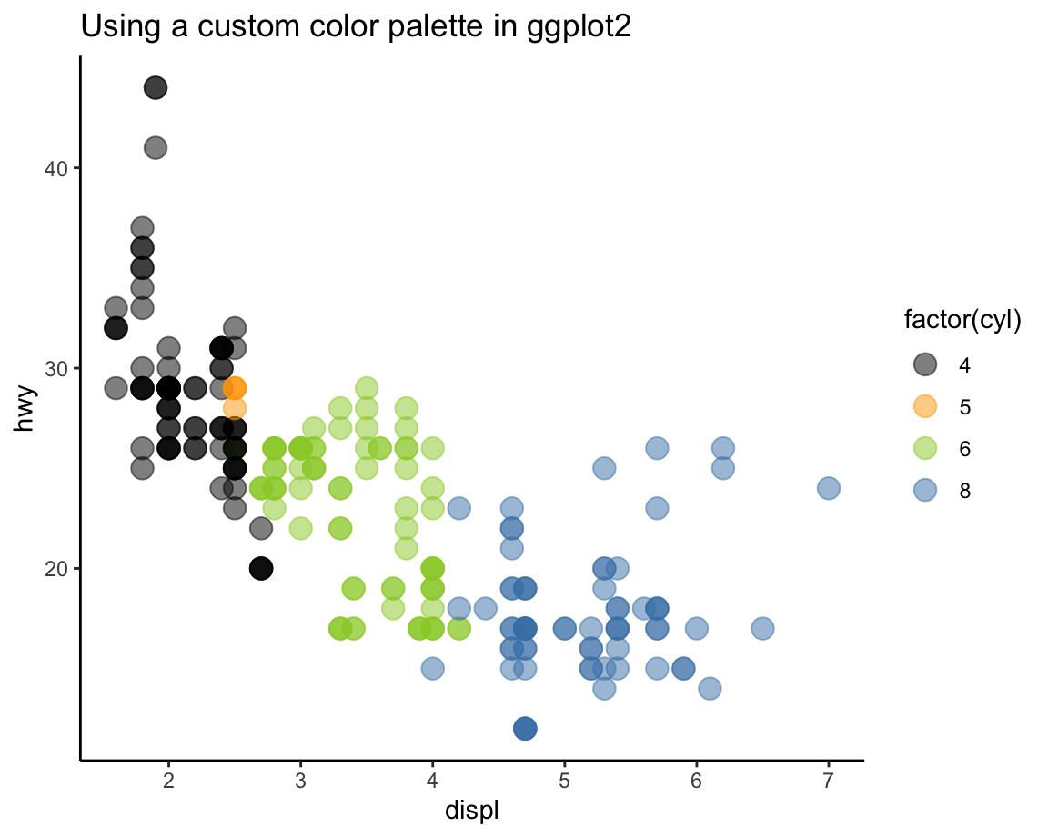
This plot illustrates the grouping function of color, which is why we defined my_pal as a qualitative color palette
(see Sections D.2.2 and D.2.3).
For base R colors, providing their names (as character strings) works just fine, as they are translated automatically into their HEX codes. For a more general solution — which also works when using colors defined by hexadecimal names, rgb() codes, or colors provided by other packages (see above) — it is safer to first define a new color palette and later access it via a color transformation function (e.g., by using the newpal() and usecol() functions of the unikn package).