7.1 Introduction
Tidy datasets are all alike
but every messy dataset is messy in its own way.Hadley Wickham (2014b, p. 2)
The notion of tidy data lies at the core of the tidyverse. Importantly, any dataset can be organized in a variety of formats. Although different formats can all contain the same data, they still differ in how easy or hard they are to work with. As we have argued in Section 3.1.1, the ease or difficulty of a particular dataset depends on the combination of our current goals, our experience and skills, and the tools (e.g., functions and packages) we are using.
The technical notion of tidy data refers to a shape that is formatted in a simple and straightforward fashion, which makes it immensely practical (e.g., easy to understand, analyze, and transform into other formats). Before defining the notion of tidy data, we first compare and contrast different sets of rectangular data that contain the same information.
7.1.1 Objectives
After working through this chapter, you will be able to:
- describe and organize the layout of data tables;
- define the notion of tidy data; and use tidyr commands to:
- separate one variable into the values of two variables;
- unite the values of two variables into one variable;
- gather values distributed over multiple columns into one variable;
- spread the values of a variable over multiple columns.
7.1.2 Varieties of tabular data
In R, rectangular data is by far the most common shape of data and typically stored as data frames or tibbles (see Sections 1.5 and Chapter 5). Importantly, such tables are internally stored as lists of atomic vectors. This means that each column of a table is a vector (of a particular type) that contains the values of a variable. Thus, whereas every column must be of one (single, homogeneous) type, every row (aka. a “case” or “observation”) can contain the values of different (heterogeneous) variables and types.
As we have seen in Section 3.1.1, the same data (e.g., the values of a variable) can be organized in many different ways. Transforming the shape of data without changing any values is known as reshaping data, as opposed to reducing or enhancing data. In this chapter, we extend the notion of “reshaping data” to different forms of rectangular tables. As a starting point, consider the following bar plot, which shows the absolute number of TB cases documented by the World Health Organization for three countries (Afghanistan, Brazil, and China) in two years (1999 and 2000):
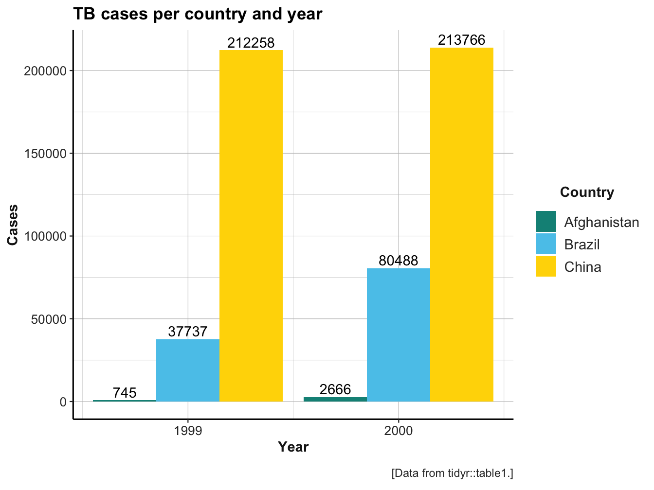
A seemingly simple question is:
- How can we represent this data in a table?
Although the amount of data in this example is very small, there are many possible ways to arrange the data in tabular form. Perhaps the most straightforward way of representing this data in a table is the following:
knitr::kable(tidyr::table4a, caption = "table4a: TB cases per country and year.")| country | 1999 | 2000 |
|---|---|---|
| Afghanistan | 745 | 2666 |
| Brazil | 37737 | 80488 |
| China | 212258 | 213766 |
The figure and table directly correspond to each other. However, when trying to use ggplot2 for re-creating the figure from the data in table4a, we realize that this is difficult.
Practice
Try recreating the above bar plot using ggplot2 with
tidyr::table4aas data. Why is this difficult?Describe a dataset that would make it easier to create this plot.
Answer
Using ggplot2 (and many other R functions) requires that we specify the independent and dependent variables. Here, the independent variables are country (with 3 instances) and year (with 2 instances). However, table4a does not contain a variable for year. Instead, each instance of the variable is represented as a column (variable). Thus, the data contains a variable (year) that is not represented as a column.
An easier dataset to create the plot would look like this:
| country | year | cases |
|---|---|---|
| Afghanistan | 1999 | 745 |
| Afghanistan | 2000 | 2666 |
| Brazil | 1999 | 37737 |
| Brazil | 2000 | 80488 |
| China | 1999 | 212258 |
| China | 2000 | 213766 |
This data contains 6 observations (cases) and 3 variables (columns): 2 independent variables (country and year) and 1 dependent variable (cases).
7.1.3 One table in many formats
Let’s consider a slightly more complicated dataset that adds the population of each country as another variable:
| country | year | cases | population |
|---|---|---|---|
| Afghanistan | 1999 | 745 | 19987071 |
| Afghanistan | 2000 | 2666 | 20595360 |
| Brazil | 1999 | 37737 | 172006362 |
| Brazil | 2000 | 80488 | 174504898 |
| China | 1999 | 212258 | 1272915272 |
| China | 2000 | 213766 | 1280428583 |
This data – available as tidyr::table1 – contains six observations (cases) and four variables (columns): Two independent variables (country and year) and two dependent variables (cases and population). (See ?tidyr::table1 for a description and source information.)
The following tables (or tibbles) all provide the same data in different formats:
- The data in
table2still contains our two dependent variables (counts of TBcasesandpopulation), but combines them in one variable (count). To signal which variable is described bycount, the data contains a new variabletypethat characterizes thecountvariable:
| country | year | type | count |
|---|---|---|---|
| Afghanistan | 1999 | cases | 745 |
| Afghanistan | 1999 | population | 19987071 |
| Afghanistan | 2000 | cases | 2666 |
| Afghanistan | 2000 | population | 20595360 |
| Brazil | 1999 | cases | 37737 |
| Brazil | 1999 | population | 172006362 |
| Brazil | 2000 | cases | 80488 |
| Brazil | 2000 | population | 174504898 |
| China | 1999 | cases | 212258 |
| China | 1999 | population | 1272915272 |
| China | 2000 | cases | 213766 |
| China | 2000 | population | 1280428583 |
A data table in this form (with several variables characterizing the cases on \(n\)-categories and one dedicated variable that provides the frequency count of each category combination) is often called a contingency table. In R, such contingency tables can also be represented in multi-dimensional data structures (of type “array,” “table” or “xtabs”).
- The data in
table3still contains the same information astable1andtable2, but collapses the information previously contained incasesandpopulationinto one variablerate. The newratevariable is represented as a ratio, which actually contains two pieces of information (numerator and denominator):
| country | year | rate |
|---|---|---|
| Afghanistan | 1999 | 745/19987071 |
| Afghanistan | 2000 | 2666/20595360 |
| Brazil | 1999 | 37737/172006362 |
| Brazil | 2000 | 80488/174504898 |
| China | 1999 | 212258/1272915272 |
| China | 2000 | 213766/1280428583 |
- The data in
table4aandtable4bsplit the information into 2 tables:table4acontains the values of TBcasesandtable4bthe counts of thepopulation. However, each sub-table splits theyearvariable into two separate variables:
| country | 1999 | 2000 |
|---|---|---|
| Afghanistan | 745 | 2666 |
| Brazil | 37737 | 80488 |
| China | 212258 | 213766 |
| country | 1999 | 2000 |
|---|---|---|
| Afghanistan | 19987071 | 20595360 |
| Brazil | 172006362 | 174504898 |
| China | 1272915272 | 1280428583 |
- The data in
table5is similar totable3in containing theratevariable (which really consists of two variables), but additionally splits up theyearinformation into two variables (noting thecenturyand a 2-digityear):
| country | century | year | rate |
|---|---|---|---|
| Afghanistan | 19 | 99 | 745/19987071 |
| Afghanistan | 20 | 00 | 2666/20595360 |
| Brazil | 19 | 99 | 37737/172006362 |
| Brazil | 20 | 00 | 80488/174504898 |
| China | 19 | 99 | 212258/1272915272 |
| China | 20 | 00 | 213766/1280428583 |
Thus, all these tables contain the same information, but differ in their layout or format. Theoretically, all these tables are equal, but some are more equal — or rather more practical — than others.
Practice
- Recreate the above bar plot using ggplot2 with
tidyr::table1as data.
7.1.4 Defining tidy data
In the previous section, we have compared many tables that contain the same data. They key motivation for tidy data is that some formats are easier to work with than others.
Definition: A tidy dataset conforms to three interrelated rules:
Each variable has its own column.
Each case/observation has its own row.
Each value has its own cell.
See the paper at https://www.jstatsoft.org/article/view/v059i10 (Wickham, 2014b) for the background of tidy data and http://r4ds.had.co.nz/tidy-data.html#fig:tidy-structure for a graphical illustration of these rules.
The three rules defining tidy data are connected, as it is impossible to only satisfy two of the three rules. This leads to a simpler set of two practical instructions for tidying a messy set of data:
A. Turn each dataset into a tibble.
B. Put each variable into a column.
Assuming that you are dealing with a single tibble, they key instruction to remember is B: Put each variable into a column.
To achieve this, we primarily need to define what should be considered as an observation (row) and what functions as a variable (column).
For instance, measuring the IQ of \(N = 100\) students twice (e.g., at the age of 10 and the age of 20) could be represented in a table that contains 100 rows (one for each student) and two separate variables for the IQ values (e.g., two columns for iq_10 and iq_20).
However, it would seem `tidier'' to represent the two IQ\ measurements as one variable (iq) per person and qualify the two measurement occasions by a key variable (age`, with two possible values 10 and 20). This table would contain two rows per person (i.e., 200 observations overall).
Although the notion of tidy data is important, it also remains — like many intuitive concepts — somewhat vague. The reason for this is that the term “variable” must be understood in a functional sense: A variable is some measure or description that we want to use as a variable in an analysis. For instance, depending on the particular task at hand, a time-related “variable” could be a particular date, or the month, year, or century that corresponds to a date. Thus, what can be considered “tidy” partly lies in the eyes of the beholder and depends on what we want to do with data, rather than on some inherent property of the data itself.
More generally, the difference between messy and tidy data depends on
(a) our goals or intended use of the data (e.g., which task do we want to address?) and
(b) the tools with which we typically carry out our tasks (e.g., which functions are we familiar with?).
Given the tools provided by R and prominent R packages (e.g., dplyr or ggplot2), it makes sense to first identify the variables of our analysis and then reshape the data so that each variable of interest is in its own column. Although this format is informationally equivalent to many alternative formats, it provides practical benefits for further transforming the data. For instance, we can easily use the variables to filter, select, group, or pivot the data to reshape or reduce it to answer our questions.
Practice
Which of the data tables in the above example (
table1totable5) are tidy? Why or why not?Is a tidy table always the most compact table (in terms of its number of cells)? (If not, provide a counterexample.)
Solution
ad 1.: In our previous examples (in Section 7.1.3), only the data of
table1was tidy, while the data intable2totable5all were messy in some way.ad 2.: Tidy data can be less compact than untidy alternative. As an example, consider and contrast the following tables:
| country | 1999 | 2000 |
|---|---|---|
| Afghanistan | 745 | 2666 |
| Brazil | 37737 | 80488 |
| China | 212258 | 213766 |
| country | year | cases |
|---|---|---|
| Afghanistan | 1999 | 745 |
| Afghanistan | 2000 | 2666 |
| Brazil | 1999 | 37737 |
| Brazil | 2000 | 80488 |
| China | 1999 | 212258 |
| China | 2000 | 213766 |
The table4a table (from the tidyr package) contains 9 cells, but is not tidy.
By contrast, a tidy version of it (that represents the year variable in its own column) contains 18 cells.
Thus, a tidy version of a table can be larger than an untidy version of the same data.
Its key benefit is not its small size, but the ease with which it can be transformed in the context of the tools provided by R.
7.1.5 Advantages of tidy data
From a theoretical viewpoint, being in a tidy format is not inherently better or worse than any of the other data formats. However, just like not all plots are equally suited to make a particular point, not all data formats are equally suited to be analyzed and transformed. As tools (like functions and packages) require data to be in a particular formats, they can only be applied if the data format fits to the requirements of the tool. Overall, tidy data has the following advantages:
Consistency: Consistent data structures make it easier to learn the tools that work with it because they have an underlying uniformity.
Vectorization: Placing variables in columns allows R’s vectorised nature to shine. For instance, the basic dplyr verbs (and most built-in R functions) work with vectors of values. That makes transforming tidy data easy and natural.
Matching data and tools: The tidyverse packages — like dplyr, ggplot2, and many others — are designed to work with tidy data.
The key advantage of tidy data is that is typically easy to work with. This does not mean that we never have to change its format. However, given the tools provided by R and the tidyverse, tidy data can easily be transformed into other formats.
Note some common misconceptions: Although tidy data tends to be a good thing, it is typically not the most compact and not necessarily the most human-readable version of a dataset. Similarly, many graphical or statistical methods require data in shapes that are not tidy (e.g., running linear regression models requires data to be in so-called long format). Again, tidy data is not an end in itself, but often a means for easily transforming data into alternative shapes. Finally, it can be difficult to decide which datasets are considered to be tidy: We usually need to interpret the semantics of the rows and columns (i.e., understand the meanings of observations and variables) to determine the tidyness of a dataset.
7.1.6 Data used
In this chapter, we will first use some variants of a simple example dataset (i.e., table1 to table5 of the tidyr package, and table6 to table8 of the ds4psy package).
However, we will also use other datasets from the dplyr and ds4psy packages, as well as revisit some data used in Tibbles (Chapter 5).
7.1.7 Getting ready
This chapter formerly assumed that you have read and worked through Chapter 12: Tidy data of the r4ds textbook (Wickham & Grolemund, 2017). It now can be read by itself, but reading Chapter 12 of r4ds is still recommended.
Please do the following to get started:
Create an R Markdown (
.Rmd) document (for instructions, see Appendix F and the templates linked in Section F.2).Structure your document by inserting headings and empty lines between different parts. Here’s an example how your initial file could look:
---
title: "Chapter 7: Tidying data"
author: "Your name"
date: "2022 July 15"
output: html_document
---

Add text or code chunks here.

# Exercises (07: Tidying data)

## Exercise 1

## Exercise 2

etc.

<!-- The end (eof). -->
Create an initial code chunk below the header of your
.Rmdfile that loads the R packages of the tidyverse (and see Section F.3.3 if you want to get rid of the messages and warnings of this chunk in your HTML output).Save your file (e.g., as
07_tidy.Rmdin the R folder of your current project) and remember saving and knitting it regularly as you keep adding content to it.
Next, we will consider four essential tidyr commands that help creating and transforming tidy data.