12.1 Introduction
‘Begin at the beginning,’ the King said gravely,
‘and go on till you come to the end: then stop.’Lewis Carroll: Alice’s Adventures in Wonderland (Chapter XII)
The king’s instruction is so general that it may seem vacuous. However, it aptly describes what happens when we program a computer, or our computer executes a rule-based process. But rather than moving from the beginning to the end, a characteristic feature of many programs is that they execute code in an iterative fashion.
To “re-iterate” something is to repeat something. In ordinary language, proceeding in an “iterative” fashion typically means to proceed step-by-step. If the steps are very similar or even identical, doing things repeatedly easily gets tedious. A notorious example of such iteration is illustrated by Figure 12.2:
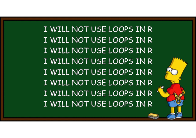
Figure 12.2: An example of punitive iteration. (Note: This post on the Learning Machines blog explains how to create this graph by using the meme package.)
In computer science, the notion of iteration implies that some code is executed repeatedly. However, doing something more than once only makes sense if some aspect of the computed code or answer can change. Thus, when repeating code, there typically is a value or object (e.g., some variable or data) that changes between consecutive iterations. More specifically, an iterative task has the general form “for each \(X\), do \(Y\).” Thus, some task \(Y\) is solved repeatedly for very input or data element \(X\). Even when the task \(Y\) always remains the same, changing the inputs or data elements \(X\) implies that iterations can yield different results. The change in \(X\) can be quite subtle. It often concerns only the value of a counter or index variable that notes the current repetition or points to some particular location in some larger data structure. In other cases, the code can contain random elements (e.g., drawing random values from some set or distribution), so that repeated executions of some task \(Y\) can yield different results.
Whereas people easily get bored or distracted when doing the same thing over and over again, computers usually do not mind and are really good at it. Thus, whenever a procedure or process requires many repetitions, computers are faster and more reliable than people.
12.1.1 Objectives
After working through this chapter, you should be able to:
- understand the notion of iteration in computer programming,
- use
forloops to iterate over sequences of a known length,
- use
whileloops to iterate over sequences of an unknown length, - use the
apply()family of functions of base R to replace some loops, - use the
map()family of functions of purrr to replace some loops.
12.1.2 Loops vs. functions
The traditional way to address issues of iteration is by repeating code in for loops. Such loops can include an arbitrary amount of code (i.e., a few lines or an entire library of programs) and execute it repeatedly.
However, the previous Chapter 11 has taught us that Functions provide another way of enclosing code: Instead of writing a loop, we could encapsulate the required code in a new function and then call this function repeatedly.
As R is a functional programming language, it provides sophisticated ways of applying functions repeatedly to data structures.
As we focus on the essentials in this book, we will primarily focus on for and while loops, and only briefly introduce the base R apply() (R Core Team, 2021) and purrr’s map() family of functions (Henry & Wickham, 2020).
12.1.3 Data used
To illustrate the notion of iteration in various type of loops, we are using various toy datasets (from the ds4psy package) in this chapter.
For instance, the dataset tb includes some information on 100 ficticious people and pi_100k contains the first 100.000 digits of pi.
12.1.4 Getting ready
This chapter formerly assumed that you have read and worked through Chapter 21: Iteration of the r4ds book (Wickham & Grolemund, 2017). It now can be read by itself, but reading Chapter 21 of r4ds is still recommended.
Please do the following to get started:
Create an R Markdown (
.Rmd) document (for instructions, see Appendix F and the templates linked in Section F.2).Structure your document by inserting headings and empty lines between different parts. Here’s an example how your initial file could look:
---
title: "Chapter 12: Iteration"
author: "Your name"
date: "2022 July 15"
output: html_document
---

Add text or code chunks here.

# Exercises (WPA12)

## Exercise 1

## Exercise 2

etc.

<!-- The end (eof). -->
Create an initial code chunk below the header of your
.Rmdfile that loads the R packages of the tidyverse (and see Section F.3.3 if you want to get rid of the messages and warnings of this chunk in your HTML output).Save your file (e.g., as
12_iteration.Rmdin the R folder of your current project) and remember saving and knitting it regularly as you keep adding content to it.