A.7 Solutions (07)

Here are the solutions of the exercises on detecting and creating tidy data of Chapter 7 (Section 7.4).
A.7.1 Exercise 1
Four messes and one tidy table
This exercise asks you to inspect some tables and turn some messy ones into tidy data.
The four tables t_1 to t_4 are available in the ds4psy package (Neth, 2022).
Alternatively, you can load csv-versions of these files from the following links:
For each of these files:
Describe the data (i.e., its dimensions, observations, variables, DVs and IVs).
Transform any non-tidy table one into a tidy one.
Verify the equality of the resulting tidy tables.
Solution
Get data files:
# from ds4psy:
t_1 <- ds4psy::t_1
t_2 <- ds4psy::t_2
t_3 <- ds4psy::t_3
t_4 <- ds4psy::t_4
1. t_1
t_1 <- ds4psy::t_1  # from ds4psy package
# t_1 <- readr::read_csv(t_1_path)  # online path
dim(t_1)  # 8 x 9
#> [1] 8 9

knitr::kable(t_1, caption = "Table t_1.")| name | gender | age | task_1 | task_2 | color | color_time | shape | shape_time |
|---|---|---|---|---|---|---|---|---|
| Ann | f | 31 | color | shape | red | 73 | circle | 64 |
| Bea | f | 18 | shape | color | blue | 18 | circle | 42 |
| Cat | f | 42 | color | shape | red | 31 | square | 41 |
| Deb | f | 18 | shape | color | blue | 35 | square | 51 |
| Ed | m | 21 | color | shape | red | 71 | circle | 44 |
| Fred | m | 63 | shape | color | blue | 56 | circle | 63 |
| Gary | m | 22 | color | shape | red | 60 | square | 98 |
| Hans | m | 31 | shape | color | blue | 40 | square | 41 |
Analysis/Description of t_1:
t_1is an 8 x 9 table, containing the data from 8 people (rows). Each person is described by her/hisname,gender, andage.The 2
task_#columns indicate the order in which the person performed 2 tasks (colorvs.shape).Both tasks exist in 2 versions (
colorinredorblue,shapeincircleorsquare).The 2 dependent variables appear to be the times (in seconds or minutes?) the person spent on each of those tasks.
Note:
The
task_2column is redundant, astask_1would suffice to specify the order of both tasks (or vice versa).A tidy dataset would feature only 1 DV of
timeand an additional key variable that specifies thetask_type(colorvs.shape).
Tidying t_1:
t_1_tidy <- t_1 %>%
  gather(key = "key", value = "time", color_time, shape_time) %>%
  separate(key, c("type", "rest"), sep = "_") %>%
  select(name:task_1, color:type, time) %>%
  arrange(name)
t_1_tidy
#> # A tibble: 16 × 8
#>    name  gender   age task_1 color shape  type   time
#>    <chr> <chr>  <dbl> <chr>  <chr> <chr>  <chr> <dbl>
#>  1 Ann   f         31 color  red   circle color    73
#>  2 Ann   f         31 color  red   circle shape    64
#>  3 Bea   f         18 shape  blue  circle color    18
#>  4 Bea   f         18 shape  blue  circle shape    42
#>  5 Cat   f         42 color  red   square color    31
#>  6 Cat   f         42 color  red   square shape    41
#>  7 Deb   f         18 shape  blue  square color    35
#>  8 Deb   f         18 shape  blue  square shape    51
#>  9 Ed    m         21 color  red   circle color    71
#> 10 Ed    m         21 color  red   circle shape    44
#> 11 Fred  m         63 shape  blue  circle color    56
#> 12 Fred  m         63 shape  blue  circle shape    63
#> 13 Gary  m         22 color  red   square color    60
#> 14 Gary  m         22 color  red   square shape    98
#> 15 Hans  m         31 shape  blue  square color    40
#> 16 Hans  m         31 shape  blue  square shape    41
2. t_2
t_2 <- ds4psy::t_2  # from ds4psy package
# t_2 <- readr::read_csv(t_2_path)  # online path
dim(t_2)  # 8 x 5
#> [1] 8 5

knitr::kable(t_2, caption = "Table t_2.")| name | details | task_1 | color_time | shape_time |
|---|---|---|---|---|
| Ann | f:31 | color | red = 73 | circle = 64 |
| Bea | f:18 | shape | blue = 18 | circle = 42 |
| Cat | f:42 | color | red = 31 | square = 41 |
| Deb | f:18 | shape | blue = 35 | square = 51 |
| Ed | m:21 | color | red = 71 | circle = 44 |
| Fred | m:63 | shape | blue = 56 | circle = 63 |
| Gary | m:22 | color | red = 60 | square = 98 |
| Hans | m:31 | shape | blue = 40 | square = 41 |
Analysis/Description of t_2:
t_2is an 8 x 5 table, and essentially are more compact version oft_1(with fewer columns).The variables
details,color_timeandshape_timeeach contain 2 variables and corresponding values.The order of tasks is specified by
task_1only (i.e., the 2nd task is implied as the other one).
Tidying t_2:
t_2_1 <- t_2 %>%
  separate(details, c("gender", "age"), sep = ":") %>%
  separate(color_time, c("color", "c_time"), sep = " = ") %>%
  separate(shape_time, c("shape", "s_time"), sep = " = ")
# t_2_1

t_2_tidy <- t_2_1 %>%
  gather(key = "key", value = "time", c_time, s_time) %>%
  separate(key, c("type", "rest"), sep = "_") %>%
  select(name:task_1, color:type, time) %>%
  arrange(name)
t_2_tidy
#> # A tibble: 16 × 8
#>    name  gender age   task_1 color shape  type  time
#>    <chr> <chr>  <chr> <chr>  <chr> <chr>  <chr> <chr>
#>  1 Ann   f      31    color  red   circle c     73
#>  2 Ann   f      31    color  red   circle s     64
#>  3 Bea   f      18    shape  blue  circle c     18
#>  4 Bea   f      18    shape  blue  circle s     42
#>  5 Cat   f      42    color  red   square c     31
#>  6 Cat   f      42    color  red   square s     41
#>  7 Deb   f      18    shape  blue  square c     35
#>  8 Deb   f      18    shape  blue  square s     51
#>  9 Ed    m      21    color  red   circle c     71
#> 10 Ed    m      21    color  red   circle s     44
#> 11 Fred  m      63    shape  blue  circle c     56
#> 12 Fred  m      63    shape  blue  circle s     63
#> 13 Gary  m      22    color  red   square c     60
#> 14 Gary  m      22    color  red   square s     98
#> 15 Hans  m      31    shape  blue  square c     40
#> 16 Hans  m      31    shape  blue  square s     41
Verify the equality of tidy tables:
Let’s make sure that t_1_tidy and t_2_tidy really are equal…
## Check equality:
# t_1_tidy
# t_2_tidy
all.equal(t_1_tidy, t_2_tidy)  # => different variable types
#> [1] "Component \"age\": Modes: numeric, character"
#> [2] "Component \"age\": target is numeric, current is character"
#> [3] "Component \"type\": 16 string mismatches"
#> [4] "Component \"time\": Modes: numeric, character"
#> [5] "Component \"time\": target is numeric, current is character"

# Create equality:
# (a) Change variable types in t_2_tidy:
t_2_tidy$gender <- as.character(t_2_tidy$gender)
t_2_tidy$age    <- as.numeric(t_2_tidy$age)
t_2_tidy$color  <- as.character(t_2_tidy$color)
t_2_tidy$shape  <- as.character(t_2_tidy$shape)
t_2_tidy$time  <- as.numeric(t_2_tidy$time)

# (b) Rename values of type:
t_2_tidy$type[t_2_tidy$type == "c"] <- "color"
t_2_tidy$type[t_2_tidy$type == "s"] <- "shape"

# t_2_tidy

## Check equality:
# t_1_tidy
# t_2_tidy
all.equal(t_1_tidy, t_2_tidy)  # => TRUE
#> [1] TRUE
3. t_3
t_3 <- ds4psy::t_3  # from ds4psy package
# t_3 <- readr::read_csv(t_3_path)  # online path
dim(t_3)  # 16 x 6
#> [1] 16  6

knitr::kable(t_3, caption = "Table t_3.")| name | gender | age | position | task | time |
|---|---|---|---|---|---|
| Ann | f | 31 | 1 | red | 73 |
| Ann | f | 31 | 2 | circle | 64 |
| Bea | f | 18 | 1 | circle | 42 |
| Bea | f | 18 | 2 | blue | 18 |
| Cat | f | 42 | 1 | red | 31 |
| Cat | f | 42 | 2 | square | 41 |
| Deb | f | 18 | 1 | square | 51 |
| Deb | f | 18 | 2 | blue | 35 |
| Ed | m | 21 | 1 | red | 71 |
| Ed | m | 21 | 2 | circle | 44 |
| Fred | m | 63 | 1 | circle | 63 |
| Fred | m | 63 | 2 | blue | 56 |
| Gary | m | 22 | 1 | red | 60 |
| Gary | m | 22 | 2 | square | 98 |
| Hans | m | 31 | 1 | square | 41 |
| Hans | m | 31 | 2 | blue | 40 |
Analysis/Description of t_3:
t_3is a 16 x 6 table.Each person appears twice, and task
position,tasktype, and tasktimeare described by 3 variables.The
taskvariable contains implicit information on task type:- values of “red” and “blue” are of type “color,”
- values of “circle” and “square” are of type “shape.”
- values of “red” and “blue” are of type “color,”
Tidying t_3:
To tidy t_3, we need to flesh out the task variable into multiple columns that denote the type, color and shape of each task.
# t_3

# Create a new variable task type:
t_3$type <- NA  # initialize variable
t_3$type[t_3$task == "red" | t_3$task == "blue"]      <- "color"
t_3$type[t_3$task == "circle" | t_3$task == "square"] <- "shape"

# Create 2 new variables color and shape:
t_3$color <- NA  # initialize variable
t_3$shape <- NA  # initialize variable
t_3$color[t_3$task == "red" | t_3$task == "blue"] <- t_3$task[t_3$task == "red" | t_3$task == "blue"]
t_3$shape[t_3$task == "circle" | t_3$task == "square"] <- t_3$task[t_3$task == "circle" | t_3$task == "square"]

t_3_tidy <- t_3 %>%
  select(name:position, type:shape, time)  # sort columns and drop task variable
t_3_tidy
#> # A tibble: 16 × 8
#>    name  gender   age position type  color shape   time
#>    <chr> <chr>  <dbl>    <dbl> <chr> <chr> <chr>  <dbl>
#>  1 Ann   f         31        1 color red   <NA>      73
#>  2 Ann   f         31        2 shape <NA>  circle    64
#>  3 Bea   f         18        1 shape <NA>  circle    42
#>  4 Bea   f         18        2 color blue  <NA>      18
#>  5 Cat   f         42        1 color red   <NA>      31
#>  6 Cat   f         42        2 shape <NA>  square    41
#>  7 Deb   f         18        1 shape <NA>  square    51
#>  8 Deb   f         18        2 color blue  <NA>      35
#>  9 Ed    m         21        1 color red   <NA>      71
#> 10 Ed    m         21        2 shape <NA>  circle    44
#> 11 Fred  m         63        1 shape <NA>  circle    63
#> 12 Fred  m         63        2 color blue  <NA>      56
#> 13 Gary  m         22        1 color red   <NA>      60
#> 14 Gary  m         22        2 shape <NA>  square    98
#> 15 Hans  m         31        1 shape <NA>  square    41
#> 16 Hans  m         31        2 color blue  <NA>      40
4. t_4
t_4 <- ds4psy::t_4  # from ds4psy package
# t_4 <- readr::read_csv(t_4_path)  # online path
dim(t_4)  # 16 x 8
#> [1] 16  8

knitr::kable(t_4, caption = "Table t_4.")| name | gender | age | position | blue | red | circle | square |
|---|---|---|---|---|---|---|---|
| Ann | f | 31 | 1 | NA | 73 | NA | NA |
| Ann | f | 31 | 2 | NA | NA | 64 | NA |
| Bea | f | 18 | 1 | NA | NA | 42 | NA |
| Bea | f | 18 | 2 | 18 | NA | NA | NA |
| Cat | f | 42 | 1 | NA | 31 | NA | NA |
| Cat | f | 42 | 2 | NA | NA | NA | 41 |
| Deb | f | 18 | 1 | NA | NA | NA | 51 |
| Deb | f | 18 | 2 | 35 | NA | NA | NA |
| Ed | m | 21 | 1 | NA | 71 | NA | NA |
| Ed | m | 21 | 2 | NA | NA | 44 | NA |
| Fred | m | 63 | 1 | NA | NA | 63 | NA |
| Fred | m | 63 | 2 | 56 | NA | NA | NA |
| Gary | m | 22 | 1 | NA | 60 | NA | NA |
| Gary | m | 22 | 2 | NA | NA | NA | 98 |
| Hans | m | 31 | 1 | NA | NA | NA | 41 |
| Hans | m | 31 | 2 | 40 | NA | NA | NA |
Analysis/Description of t_4:
t_4is a 16 x 8 table.Each person appears twice, and the task
positionis encoded by a variable.The task
timeinformation is distributed across 4 columns (blue,red,circle, andsquare), which also encode tasktypeandcolororshape.
Tidying t_4:
Here are 2 different solutions for tidying t_4:
t_4
#> # A tibble: 16 × 8
#>    name  gender   age position  blue   red circle square
#>    <chr> <chr>  <dbl>    <dbl> <dbl> <dbl>  <dbl>  <dbl>
#>  1 Ann   f         31        1    NA    73     NA     NA
#>  2 Ann   f         31        2    NA    NA     64     NA
#>  3 Bea   f         18        1    NA    NA     42     NA
#>  4 Bea   f         18        2    18    NA     NA     NA
#>  5 Cat   f         42        1    NA    31     NA     NA
#>  6 Cat   f         42        2    NA    NA     NA     41
#>  7 Deb   f         18        1    NA    NA     NA     51
#>  8 Deb   f         18        2    35    NA     NA     NA
#>  9 Ed    m         21        1    NA    71     NA     NA
#> 10 Ed    m         21        2    NA    NA     44     NA
#> 11 Fred  m         63        1    NA    NA     63     NA
#> 12 Fred  m         63        2    56    NA     NA     NA
#> 13 Gary  m         22        1    NA    60     NA     NA
#> 14 Gary  m         22        2    NA    NA     NA     98
#> 15 Hans  m         31        1    NA    NA     NA     41
#> 16 Hans  m         31        2    40    NA     NA     NA

# Solution 1: Gather 4 time variables + filter out non-NA cases: --------
t_4_mod <- t_4 %>%
  gather(key = "task", value = "time", blue:square) %>%
  filter(!is.na(time)) %>%
  arrange(name, position)
t_4_mod
#> # A tibble: 16 × 6
#>    name  gender   age position task    time
#>    <chr> <chr>  <dbl>    <dbl> <chr>  <dbl>
#>  1 Ann   f         31        1 red       73
#>  2 Ann   f         31        2 circle    64
#>  3 Bea   f         18        1 circle    42
#>  4 Bea   f         18        2 blue      18
#>  5 Cat   f         42        1 red       31
#>  6 Cat   f         42        2 square    41
#>  7 Deb   f         18        1 square    51
#>  8 Deb   f         18        2 blue      35
#>  9 Ed    m         21        1 red       71
#> 10 Ed    m         21        2 circle    44
#> 11 Fred  m         63        1 circle    63
#> 12 Fred  m         63        2 blue      56
#> 13 Gary  m         22        1 red       60
#> 14 Gary  m         22        2 square    98
#> 15 Hans  m         31        1 square    41
#> 16 Hans  m         31        2 blue      40

# Verify that t_4_mod is equal to t_3 (from above):
all.equal(t_3, t_4_mod)
#> [1] "Attributes: < Length mismatch: comparison on first 2 components >"
#> [2] "Attributes: < Component \"class\": 3 string mismatches >"
#> [3] "Length mismatch: comparison on first 6 components"

# From here on, cleaning t_4_mod is equal to cleaning t_3 (see above).


# Solution 2: Fleshing out info in 4 time columns by hand (base R): --------
t_4[is.na(t_4)] <- 0  # replace NA values by values of 0
t_4$time <- t_4$blue + t_4$red + t_4$circle + t_4$square

# Create 2 new variables color and shape:
t_4$color <- NA  # initialize variable
t_4$shape <- NA  # initialize variable
t_4$color[t_4$blue > 0] <- "blue"
t_4$color[t_4$red > 0] <- "red"
t_4$shape[t_4$circle > 0] <- "circle"
t_4$shape[t_4$square > 0] <- "square"

# Create a new variable task type:
t_4$type <- NA  # initialize variable
t_4$type[!is.na(t_4$color)] <- "color"
t_4$type[!is.na(t_4$shape)] <- "shape"

t_4_tidy <- t_4 %>%
  select(name:position, type, color, shape, time)
t_4_tidy
#> # A tibble: 16 × 8
#>    name  gender   age position type  color shape   time
#>    <chr> <chr>  <dbl>    <dbl> <chr> <chr> <chr>  <dbl>
#>  1 Ann   f         31        1 color red   <NA>      73
#>  2 Ann   f         31        2 shape <NA>  circle    64
#>  3 Bea   f         18        1 shape <NA>  circle    42
#>  4 Bea   f         18        2 color blue  <NA>      18
#>  5 Cat   f         42        1 color red   <NA>      31
#>  6 Cat   f         42        2 shape <NA>  square    41
#>  7 Deb   f         18        1 shape <NA>  square    51
#>  8 Deb   f         18        2 color blue  <NA>      35
#>  9 Ed    m         21        1 color red   <NA>      71
#> 10 Ed    m         21        2 shape <NA>  circle    44
#> 11 Fred  m         63        1 shape <NA>  circle    63
#> 12 Fred  m         63        2 color blue  <NA>      56
#> 13 Gary  m         22        1 color red   <NA>      60
#> 14 Gary  m         22        2 shape <NA>  square    98
#> 15 Hans  m         31        1 shape <NA>  square    41
#> 16 Hans  m         31        2 color blue  <NA>      40
Verify the equality of tidy tables:
Let’s make sure that t_3_tidy and t_4_tidy really are equal…
# Verify equality: --------
all.equal(t_3_tidy, t_4_tidy)
#> [1] TRUE
A.7.2 Exercise 2
Moving stocks from wide to long to wide
Let’s enter and transform some stock-related data.74
The following table shows the start and end price of three stocks on three days (d1, d2, d3):
| stock | d1_start | d1_end | d2_start | d2_end | d3_start | d3_end |
|---|---|---|---|---|---|---|
| Amada | 2.5 | 3.6 | 3.5 | 4.2 | 4.4 | 2.8 |
| Betix | 3.3 | 2.9 | 3.0 | 2.1 | 2.3 | 2.5 |
| Cevis | 4.2 | 4.8 | 4.6 | 3.1 | 3.2 | 3.7 |
Create a tibble
stthat contains this data in this (wide) format.Transform
stinto a longer tablest_longthat contains 18 rows and only one numeric variable for all stock prices. Adjust this table so that thedayandtimeappear as 2 separate columns.Create a (line) graph that shows the three stocks’
endprices (on the y-axis) over the three days (on the x-axis).Spread
st_longinto a wider table that containsstartandendprices as two distinct variables (columns) for each stock and day.
Solution
# library(tidyverse)

# 1. Enter stock data (in wide format) as a tibble: ----
st <- tribble(
  ~stock, ~d1_start, ~d1_end, ~d2_start, ~d2_end, ~d3_start, ~d3_end,
  #-----|----------|--------|----------|--------|----------|--------|
  "Amada",   2.5,     3.6,    3.5,       4.2,      4.4,       2.8,
  "Betix",   3.3,     2.9,    3.0,       2.1,      2.3,       2.5,
  "Cevis",   4.2,     4.8,    4.6,       3.1,      3.2,       3.7
)
dim(st)
#> [1] 3 7

## Note data structure:
## 2 nested factors: day (1 to 3), type (start or end).

# 2. Change from wide to long format ----
#    that contains the day (d1, d2, d3) and type (start vs. end) as separate columns:
st_long <- st %>%
  gather(d1_start:d3_end, key = "key", value = "val") %>%
  separate(key, into = c("day", "time")) %>%
  arrange(stock, day, time) # optional: arrange rows
st_long
#> # A tibble: 18 × 4
#>    stock day   time    val
#>    <chr> <chr> <chr> <dbl>
#>  1 Amada d1    end     3.6
#>  2 Amada d1    start   2.5
#>  3 Amada d2    end     4.2
#>  4 Amada d2    start   3.5
#>  5 Amada d3    end     2.8
#>  6 Amada d3    start   4.4
#>  7 Betix d1    end     2.9
#>  8 Betix d1    start   3.3
#>  9 Betix d2    end     2.1
#> 10 Betix d2    start   3
#> 11 Betix d3    end     2.5
#> 12 Betix d3    start   2.3
#> 13 Cevis d1    end     4.8
#> 14 Cevis d1    start   4.2
#> 15 Cevis d2    end     3.1
#> 16 Cevis d2    start   4.6
#> 17 Cevis d3    end     3.7
#> 18 Cevis d3    start   3.2

# 3. Plot the end values (on the y-axis) of the 3 stocks over 3 days (x-axis): ----
st_long %>%
  filter(time == "end") %>%
  ggplot(aes(x = day, y = val, color = stock, shape = stock)) +
  geom_point(size = 5) +
  geom_line(aes(group = stock), size = 1, alpha = 2/3) +
  labs(title = "End prices of each stock (by day)",
       x = "Day", y = "End price",
       shape = "Stock:", color = "Stock:") +
  # scale_color_manual(values = c("steelblue", "firebrick", "forestgreen")) +
  scale_color_manual(values = usecol(pal = c(Seeblau, Seegruen, Pinky))) +  # assuming library("unikn")
  theme_bw()

# 4. Change st_long into a wider format that lists start and end as 2 distinct variables (columns): ----
st_long %>%
  spread(key = time, value = val) %>%
  mutate(day_nr = parse_integer(str_sub(day, 2, 2))) # optional: get day_nr as integer variable
#> # A tibble: 9 × 5
#>   stock day     end start day_nr
#>   <chr> <chr> <dbl> <dbl>  <int>
#> 1 Amada d1      3.6   2.5      1
#> 2 Amada d2      4.2   3.5      2
#> 3 Amada d3      2.8   4.4      3
#> 4 Betix d1      2.9   3.3      1
#> 5 Betix d2      2.1   3        2
#> 6 Betix d3      2.5   2.3      3
#> 7 Cevis d1      4.8   4.2      1
#> 8 Cevis d2      3.1   4.6      2
#> 9 Cevis d3      3.7   3.2      3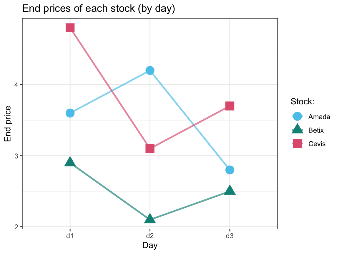
A.7.3 Exercise 3
In this exercise, we use tidyr to solve a problem that prevented us from creating a plot in the tibble chapter (Chapter 5).
A posPsy tibble reloaded
In Exercise 3 of Chapter 5,
we created a tibble of mean depression scores (my_tbl and my_tbl_2) in 2 different ways (by entering the data directly into R with tibble() and by using dplyr to compute a summary table from the posPsy_wide data).
| intervention | mn_cesd_0 | mn_cesd_1 | mn_cesd_2 | mn_cesd_3 | mn_cesd_4 | mn_cesd_5 |
|---|---|---|---|---|---|---|
| 1 | 15.1 | 15.3 | 13.6 | 12.0 | 11.2 | 13.5 |
| 2 | 16.2 | 14.6 | 11.4 | 12.5 | 13.4 | 14.6 |
| 3 | 16.1 | 12.3 | 14.8 | 13.9 | 14.9 | 13.0 |
| 4 | 12.8 | 9.9 | 9.5 | 9.1 | 7.7 | 10.2 |
See Section B.1 of Appendix B for details on the data.
When trying to create a plot that shows the trends of mean depression scores (over different occasions by intervention) we noted that it is impossible to directly plot the values of my_tbl_2. For plotting the mean depression scores with ggplot we would need these scores as 1 dependent variable, rather than as six different variables.
Earlier, we solved this problem by creating an alternative tibble my_tbl_3 — which expressed mean_cesd as a function of occasion and intervention (in long format) — from the raw data in posPsy_long. Given our new skills in tidyr, we now are in a position to transform my_tbl_2 (or my_tbl) into the required format of my_tbl_3. Thus, your task is:
- Re-create one of the original tibbles (either
my_tblormy_tbl_2) and use tidyr to transform it into the long format ofmy_tbl_3.
Solution
# Load data: ----
posPsy_wide <- ds4psy::posPsy_wide  # from ds4psy package
# posPsy_wide <- read_csv(file = "http://rpository.com/ds4psy/data/posPsy_data_wide.csv")  # online
# dim(posPsy_wide)  # 295 294

# Re-create tibble: ----
my_tbl_2 <- posPsy_wide %>%
  group_by(intervention) %>%
  summarise(mn_cesd_0 = round(mean(cesdTotal.0, na.rm = TRUE), 1),
            mn_cesd_1 = round(mean(cesdTotal.1, na.rm = TRUE), 1),
            mn_cesd_2 = round(mean(cesdTotal.2, na.rm = TRUE), 1),
            mn_cesd_3 = round(mean(cesdTotal.3, na.rm = TRUE), 1),
            mn_cesd_4 = round(mean(cesdTotal.4, na.rm = TRUE), 1),
            mn_cesd_5 = round(mean(cesdTotal.5, na.rm = TRUE), 1) )
# my_tbl_2

# Transform from wide into long format: ----
my_tbl_3 <- my_tbl_2 %>%
  gather(key = "key", value = "mean_cesd", mn_cesd_0:mn_cesd_5) %>%
  separate(key, c("mn", "cesd", "occasion"), sep = "_") %>%
  select(occasion, intervention, mean_cesd)
# my_tbl_3

# Change some variable types:
my_tbl_3$occasion     <- as.integer(my_tbl_3$occasion)    # as integer
my_tbl_3$intervention <- as.factor(my_tbl_3$intervention) # as factor

# Check:
my_tbl_3
#> # A tibble: 24 × 3
#>    occasion intervention mean_cesd
#>       <int> <fct>            <dbl>
#>  1        0 1                 15.1
#>  2        0 2                 16.2
#>  3        0 3                 16.1
#>  4        0 4                 12.8
#>  5        1 1                 15.3
#>  6        1 2                 14.6
#>  7        1 3                 12.3
#>  8        1 4                  9.9
#>  9        2 1                 13.6
#> 10        2 2                 11.4
#> # … with 14 more rows- Now do the reverse:
Use the long version
my_tbl_3to (re-)create a wider versionmy_tbl_4that is equal tomy_tbl_2.
Solution
my_tbl_4 <- my_tbl_3 %>%
  spread(key = occasion, value = mean_cesd)
my_tbl_4
#> # A tibble: 4 × 7
#>   intervention   `0`   `1`   `2`   `3`   `4`   `5`
#>   <fct>        <dbl> <dbl> <dbl> <dbl> <dbl> <dbl>
#> 1 1             15.1  15.3  13.6  12    11.2  13.5
#> 2 2             16.2  14.6  11.4  12.5  13.4  14.6
#> 3 3             16.1  12.3  14.8  13.9  14.9  13
#> 4 4             12.8   9.9   9.5   9.1   7.7  10.2

# Change names of some variables (columns 2:7):
names(my_tbl_4)[2:ncol(my_tbl_4)] <- paste0("mn_cesd_", names(my_tbl_4)[2:ncol(my_tbl_4)])

# Change some variable types:
my_tbl_4$intervention <- as.double(my_tbl_4$intervention) # back to number

## Verify equality:
# my_tbl_4
# my_tbl_2
all.equal(my_tbl_4, my_tbl_2)
#> [1] TRUE
A.7.4 Exercise 4
Wide and long psychology
In previous chapters, we have seen 2 sets of data for the positive psychology experiment:
ds4psy::posPsy_longwith 990 x 50 variables (aka.posPsy_AHI_CESD_corrected.csv, available online at http://rpository.com/ds4psy/data/posPsy_AHI_CESD_corrected.csv)ds4psy::posPsy_widewith 295 x 294 variables (aka.posPsy_data_wide.csv, available online at http://rpository.com/ds4psy/data/posPsy_data_wide.csv)
(See Section B.1 of Appendix B for details on the data.)
Both of these datasets contain the same information, but one is in long format and one in wide format. With tidyr, we are able to transform the long format into wide format (and vice versa) on our own.
1. From long to wide
Load the file
posPsy_AHI_CESD_corrected.csvinto a tibbleposPsy_long. To make things simpler, drop all columns exceptid,occasion,intervention, andahiTotal.Transform the resulting table from long to wide format (spreading
ahiTotalvalues over differentoccasions).
Solution
## Load data: ----
posPsy_long <- ds4psy::posPsy_long  # from ds4psy package
# posPsy_long <- read_csv(file = "http://rpository.com/ds4psy/data/posPsy_AHI_CESD_corrected.csv")  # online
dim(posPsy_long)  # 990 x 50
#> [1] 990  50

## Drop most colums: ----
df_long <- posPsy_long %>%
  select(id, occasion, intervention, ahiTotal)
## Check:
# df_long
dim(df_long)  # 990 x 4
#> [1] 990   4

## Spread to wide format: ----
df_wide <- df_long %>%
  spread(occasion, ahiTotal, convert = TRUE)

## Check:
dim(df_wide)  # 295 x 8
#> [1] 295   8

# Fix some variable names:
names(df_wide)[3:8] <- paste0("occ_", names(df_wide)[3:8])

## Check:
df_wide
#> # A tibble: 295 × 8
#>       id intervention occ_0 occ_1 occ_2 occ_3 occ_4 occ_5
#>    <dbl>        <dbl> <int> <int> <int> <int> <int> <int>
#>  1     1            4    63    73    NA    NA    NA    NA
#>  2     2            1    73    89    89    93    80    77
#>  3     3            4    77    NA    85    NA    NA    NA
#>  4     4            3    60    67    NA    56    61    NA
#>  5     5            2    41    41    47    47    47    NA
#>  6     6            1    62    NA    67    66    NA    NA
#>  7     7            3    67    NA    NA    NA    NA    NA
#>  8     8            2    59    45    38    48    43    NA
#>  9     9            1    48    NA    NA    NA    NA    NA
#> 10    10            2    58    NA    NA    NA    NA    NA
#> # … with 285 more rows
2. From wide to long
Load the file
posPsy_data_wide.csvinto a tibbleposPsy_wideand drop all variables that contain values of individual happiness or depression items (i.e., all score variables not containing “Total” in their names).Then transform this wide format tibble into long format. Your result table should contain all demographic information (in separate columns), the type of scale (ahiTotal vs. cesdTotal), number of
occasion(0 to 5), and the scalevalue(as dependent variable).
Hint: First gather all Total variables into a single value variable, then separate the key column into 2 variables scale and occasion.
Solution
## Load data: ----
posPsy_wide <- read_csv(file = "http://rpository.com/ds4psy/data/posPsy_data_wide.csv")  # online
dim(posPsy_wide)  # 295 x 294
#> [1] 295 294

## Drop unnecessary columns and gather: ----
df_long <- posPsy_wide %>%
  # drop unnecessary columns:
  select(id, intervention, sex, age, educ, income, contains("Total")) %>%
  gather(-id, -intervention, -sex, -age, -educ, -income,
         key = "score.occasion",
         value = "value")
## Check:
dim(df_long)  # 3540 x 8
#> [1] 3540    8
# df_long

## Separate key column score.occasion: ----
df_long <- df_long %>%
  separate(score.occasion,
           into = c("scale", "occasion"))
## Check:
dim(df_long)  # 3540 x 9
#> [1] 3540    9
# df_long

# Fix some variables:
df_long$occasion <- as.integer(df_long$occasion)

df_long
#> # A tibble: 3,540 × 9
#>       id intervention   sex   age  educ income scale    occasion value
#>    <dbl>        <dbl> <dbl> <dbl> <dbl>  <dbl> <chr>       <int> <dbl>
#>  1     1            4     2    35     5      3 ahiTotal        0    63
#>  2     2            1     1    59     1      1 ahiTotal        0    73
#>  3     3            4     1    51     4      3 ahiTotal        0    77
#>  4     4            3     1    50     5      2 ahiTotal        0    60
#>  5     5            2     2    58     5      2 ahiTotal        0    41
#>  6     6            1     1    31     5      1 ahiTotal        0    62
#>  7     7            3     1    44     5      2 ahiTotal        0    67
#>  8     8            2     1    57     4      2 ahiTotal        0    59
#>  9     9            1     1    36     4      3 ahiTotal        0    48
#> 10    10            2     1    45     4      3 ahiTotal        0    58
#> # … with 3,530 more rows
A.7.5 Exercise 5
Plotting relatives
This exercise relies on the main dataset for false positive psychology (see Section B.2 of Appendix B for details on the data and corresponding information):
- Load the data file
falsePosPsy_all(78 x 19 variables):
# Import dataset
falsePosPsy_all <- ds4psy::falsePosPsy_all  # from ds4psy package
# falsePosPsy_all <- read_csv("http://rpository.com/ds4psy/data/falsePosPsy_all.csv")  # online

# Check:
dim(falsePosPsy_all)  # 78 x 19
#> [1] 78 19
# falsePosPsy_all
Parents’ age?
Let’s see whether we can detect some relationship between the parents’ age values.
- Plot the relationship between the age values of each participant’s
dadandmom(e.g., as a scatterplot).
Solution
df <- falsePosPsy_all  # copy the data

ggplot(df, aes(x = dad, y = mom)) +
  geom_point(alpha = 1/2) +
  geom_smooth(se = FALSE, color = unikn::Seeblau) +  # assuming library('unikn')
  theme_bw()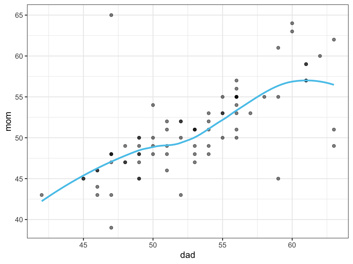
- Plot the age distributions of moms vs. dads (i.e., the distributions of age values among moms vs. dads) using histograms or
geom_bar.
(Hint: As both ages are in two separate variables, you need to use gather to collect the ages of both parents in one variable.)
Solution
df %>%
  gather(key = "parent", value = "age", dad, mom) %>%
  select(study:aged365, parent, age) %>%
  ggplot(aes(x = age, fill = parent)) +
  geom_bar(position = "dodge") +
  facet_wrap(~parent) +
  scale_y_continuous(limits = c(0, 10),
                     breaks = c(1:10)) +
  labs(title = "Age distributions of parents") +
  # scale_fill_manual(values = c("steelblue3", "sienna2")) +
  scale_fill_manual(values = usecol(c(Seeblau, Peach))) +  # assuming library('unikn')
  theme_bw()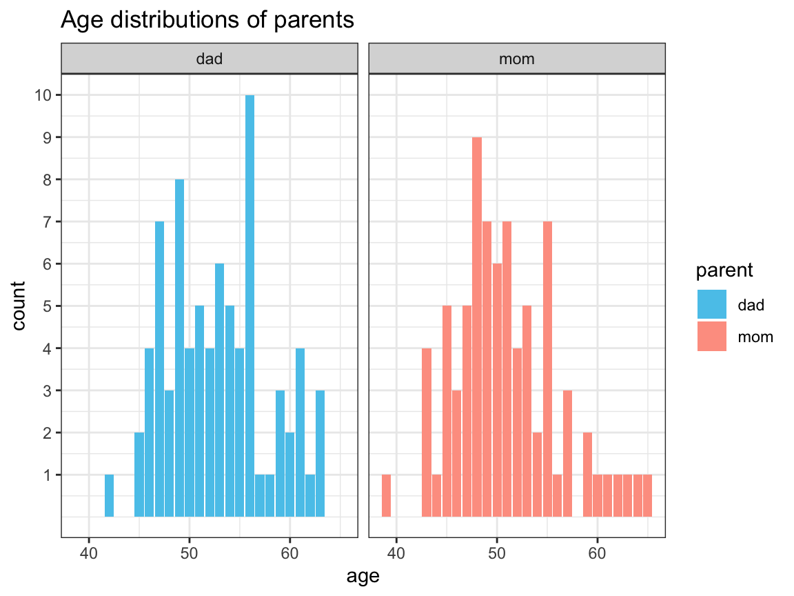
- Can you think of a way of plotting the relationship between (or difference between) the age of both parents for each participant?
(Hint: Again, you need to use gather to collect the ages of both parents into one variable.)
Solution
df_long <- df %>%
  mutate(similar_ages = (abs(dad - mom) < 5)) %>%  # similar_ages if difference below 5 years
  select(study:mom, similar_ages) %>%
  gather(key = "parent", value = "age", dad:mom)
# df_long

ggplot(df_long, aes(x = parent, y = age)) +
  geom_line(aes(group = ID, color = similar_ages), alpha = .3, size = 2) +
  facet_grid(~similar_ages) +
  labs(title = "Relations between parents' ages") +
  # scale_color_manual(values = c("red3", "black")) +
  scale_color_manual(values = usecol(c(Bordeaux, Petrol))) +  # assuming library('unikn')
  theme_bw()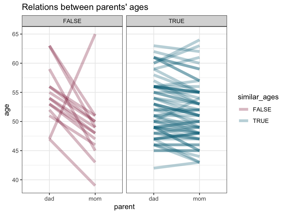
We see that most parents are of a similar age (i.e., have an age difference smaller than 5 years). Of the parents with larger age differences it is mostly the dads older than the moms, except for one case in the other direction.
A.7.6 Exercise 6
Experiment with wider data
This is a bonus task — for the ambitious or curious — which requires transforming a dataset with multiple dependent variables into tidy data.
This task extends beyond the scope of the current chapter, but can be solved with our current base R and tidyverse commands.
(See Section 7.2.6 for additional information.)
Data
The data table exp_wide contains data from \(n = 10\) participants.
Each participant completed two tasks (and the task position p was randomized).
For each task, we measured two dependent variables: The correctness c of the response, and the time t (in msec) to complete the task:
| subj | p_1 | p_2 | c_1 | c_2 | t_1 | t_2 |
|---|---|---|---|---|---|---|
| 1 | 1 | 2 | FALSE | FALSE | 4873.7 | 9230.0 |
| 2 | 1 | 2 | FALSE | FALSE | 3963.9 | 2948.8 |
| 3 | 2 | 1 | FALSE | TRUE | 2868.4 | 8348.3 |
| 4 | 2 | 1 | FALSE | FALSE | 2561.3 | 1290.2 |
| 5 | 1 | 2 | TRUE | FALSE | 5762.2 | 9330.7 |
| 6 | 1 | 2 | FALSE | FALSE | 4873.7 | 9230.0 |
| 7 | 2 | 1 | FALSE | TRUE | 3963.9 | 2948.8 |
| 8 | 1 | 2 | TRUE | TRUE | 2868.4 | 8348.3 |
| 9 | 2 | 1 | TRUE | TRUE | 2561.3 | 1290.2 |
| 10 | 2 | 1 | TRUE | FALSE | 5762.2 | 9330.7 |
Tasks
Import the data from
ds4psy::exp_wide(or http://rpository.com/ds4psy/data/exp_wide.csv) into a tibbleexp_wide.Use 2 different ways to transform (or reshape)
exp_wideinto a table of tidy dataexp_tidy.Verify the equality of both solutions.
Solution
- Solution 1 by using
stats::reshape():
Note that reshape() assumes a data frame, rather than a tibble, which is why we will convert it with as.data.frame() and convert the result into a tibble with as_tibble().
## Load data: ----
exp_wide <- ds4psy::exp_wide  # from ds4psy package
# exp_wide <- readr::read_csv(file = "http://rpository.com/ds4psy/data/exp_wide.csv")  # online
dim(exp_wide)  # 10 x 7
#> [1] 10  7

# Turn into a data frame:
exp_wide <- as.data.frame(exp_wide)

## Use reshape to transform into long format:
exp_long <- stats::reshape(data = exp_wide,
                           direction = "long",
                           varying = list(p = 2:3, # 1st set of variables to combine into 1
                                          c = 4:5, # 2nd set of variables to combine into 1
                                          t = 6:7),
                           v.names = c("position", "correct", "time")
)

exp_tidy_1 <- exp_long %>%
  select(subj, position, correct, time) %>%
  arrange(subj, position)

exp_tidy_1 <- as_tibble(exp_tidy_1)
exp_tidy_1
#> # A tibble: 20 × 4
#>     subj position correct  time
#>    <dbl>    <dbl> <lgl>   <dbl>
#>  1     1        1 FALSE   4874.
#>  2     1        2 FALSE   9230
#>  3     2        1 FALSE   3964.
#>  4     2        2 FALSE   2949.
#>  5     3        1 TRUE    8348.
#>  6     3        2 FALSE   2868.
#>  7     4        1 FALSE   1290.
#>  8     4        2 FALSE   2561.
#>  9     5        1 TRUE    5762.
#> 10     5        2 FALSE   9331.
#> 11     6        1 FALSE   4874.
#> 12     6        2 FALSE   9230
#> 13     7        1 TRUE    2949.
#> 14     7        2 FALSE   3964.
#> 15     8        1 TRUE    2868.
#> 16     8        2 TRUE    8348.
#> 17     9        1 TRUE    1290.
#> 18     9        2 TRUE    2561.
#> 19    10        1 FALSE   9331.
#> 20 10 2 TRUE 5762.- Solution 2 by using multiple tidyr commands:
## Load data: ----
exp_wide <- ds4psy::exp_wide  # from ds4psy package
# exp_wide <- readr::read_csv(file = "http://rpository.com/ds4psy/data/exp_wide.csv")  # online
dim(exp_wide)  # 10 x 7
#> [1] 10  7
exp_wide
#> # A tibble: 10 × 7
#>     subj   p_1   p_2 c_1   c_2     t_1   t_2
#>    <dbl> <dbl> <dbl> <lgl> <lgl> <dbl> <dbl>
#>  1     1     1     2 FALSE FALSE 4874. 9230
#>  2     2     1     2 FALSE FALSE 3964. 2949.
#>  3     3     2     1 FALSE TRUE  2868. 8348.
#>  4     4     2     1 FALSE FALSE 2561. 1290.
#>  5     5     1     2 TRUE  FALSE 5762. 9331.
#>  6     6     1     2 FALSE FALSE 4874. 9230
#>  7     7     2     1 FALSE TRUE  3964. 2949.
#>  8     8     1     2 TRUE  TRUE  2868. 8348.
#>  9     9     2     1 TRUE  TRUE  2561. 1290.
#> 10    10     2     1 TRUE  FALSE 5762. 9331.

## Gather all 6 dependent variables (from wide into long format): --------
exp_long <- exp_wide %>%
  gather(key = "key", value = "value", p_1:t_2) %>%
  separate(col = key, into = c("var", "pos"))
exp_long
#> # A tibble: 60 × 4
#>     subj var   pos   value
#>    <dbl> <chr> <chr> <dbl>
#>  1     1 p     1         1
#>  2     2 p     1         1
#>  3     3 p     1         2
#>  4     4 p     1         2
#>  5     5 p     1         1
#>  6     6 p     1         1
#>  7     7 p     1         2
#>  8     8 p     1         1
#>  9     9 p     1         2
#> 10    10 p     1         2
#> # … with 50 more rows

## Deal with 3 sub-tables (of different DVs): --------

# 1st slice of 20 rows: Position information
exp_pos <- exp_long %>%
  filter(var == "p") %>%   # filter 20 rows with position info
  select(subj, pos, value) %>%
  rename(position = value) %>%
  arrange(subj, pos)  # ensure order
exp_pos
#> # A tibble: 20 × 3
#>     subj pos   position
#>    <dbl> <chr>    <dbl>
#>  1     1 1            1
#>  2     1 2            2
#>  3     2 1            1
#>  4     2 2            2
#>  5     3 1            2
#>  6     3 2            1
#>  7     4 1            2
#>  8     4 2            1
#>  9     5 1            1
#> 10     5 2            2
#> 11     6 1            1
#> 12     6 2            2
#> 13     7 1            2
#> 14     7 2            1
#> 15     8 1            1
#> 16     8 2            2
#> 17     9 1            2
#> 18     9 2            1
#> 19    10 1            2
#> 20    10 2            1

# 2nd slice of 20 rows: Correctness information
exp_cor <- exp_long %>%
  filter(var == "c") %>%  # filter 20 rows with correctness info
  select(subj, pos, value) %>%
  mutate(correct = as.logical(value)) %>%  # correct as Boolean value!
  select(subj, pos, correct) %>%
  arrange(subj, pos)  # ensure order
exp_cor
#> # A tibble: 20 × 3
#>     subj pos   correct
#>    <dbl> <chr> <lgl>
#>  1     1 1     FALSE
#>  2     1 2     FALSE
#>  3     2 1     FALSE
#>  4     2 2     FALSE
#>  5     3 1     FALSE
#>  6     3 2     TRUE
#>  7     4 1     FALSE
#>  8     4 2     FALSE
#>  9     5 1     TRUE
#> 10     5 2     FALSE
#> 11     6 1     FALSE
#> 12     6 2     FALSE
#> 13     7 1     FALSE
#> 14     7 2     TRUE
#> 15     8 1     TRUE
#> 16     8 2     TRUE
#> 17     9 1     TRUE
#> 18     9 2     TRUE
#> 19    10 1     TRUE
#> 20    10 2     FALSE

# 3rd slice of 20 rows: Time information
exp_time <- exp_long %>%
  filter(var == "t") %>%
  select(subj, pos, value) %>%
  mutate(time = as.numeric(value)) %>%  # time as numeric value!
  select(subj, pos, time) %>%
  arrange(subj, pos)  # ensure order
exp_time
#> # A tibble: 20 × 3
#>     subj pos    time
#>    <dbl> <chr> <dbl>
#>  1     1 1     4874.
#>  2     1 2     9230
#>  3     2 1     3964.
#>  4     2 2     2949.
#>  5     3 1     2868.
#>  6     3 2     8348.
#>  7     4 1     2561.
#>  8     4 2     1290.
#>  9     5 1     5762.
#> 10     5 2     9331.
#> 11     6 1     4874.
#> 12     6 2     9230
#> 13     7 1     3964.
#> 14     7 2     2949.
#> 15     8 1     2868.
#> 16     8 2     8348.
#> 17     9 1     2561.
#> 18     9 2     1290.
#> 19    10 1     5762.
#> 20    10 2     9331.


# Combine all 3 sub-tables again: --------
exp_pos_cor      <- left_join(exp_pos, exp_cor)
exp_pos_cor_time <- left_join(exp_pos_cor, exp_time)

# Select and arrange:
exp_tidy_2 <- exp_pos_cor_time %>%
  select(subj, position, correct, time) %>%
  arrange(subj, position)

exp_tidy_2
#> # A tibble: 20 × 4
#>     subj position correct  time
#>    <dbl>    <dbl> <lgl>   <dbl>
#>  1     1        1 FALSE   4874.
#>  2     1        2 FALSE   9230
#>  3     2        1 FALSE   3964.
#>  4     2        2 FALSE   2949.
#>  5     3        1 TRUE    8348.
#>  6     3        2 FALSE   2868.
#>  7     4        1 FALSE   1290.
#>  8     4        2 FALSE   2561.
#>  9     5        1 TRUE    5762.
#> 10     5        2 FALSE   9331.
#> 11     6        1 FALSE   4874.
#> 12     6        2 FALSE   9230
#> 13     7        1 TRUE    2949.
#> 14     7        2 FALSE   3964.
#> 15     8        1 TRUE    2868.
#> 16     8        2 TRUE    8348.
#> 17     9        1 TRUE    1290.
#> 18     9        2 TRUE    2561.
#> 19    10        1 FALSE   9331.
#> 20 10 2 TRUE 5762.- Verify the equality of both solutions:
all.equal(exp_tidy_1, exp_tidy_2)  # TRUE (qed).
#>  [1] "Attributes: < Names: 1 string mismatch >"
#>  [2] "Attributes: < Length mismatch: comparison on first 2 components >"
#>  [3] "Attributes: < Component 2: Modes: list, numeric >"
#>  [4] "Attributes: < Component 2: names for target but not for current >"
#>  [5] "Attributes: < Component 2: Length mismatch: comparison on first 4 components >"
#>  [6] "Attributes: < Component 2: Component 1: Modes: list, numeric >"
#>  [7] "Attributes: < Component 2: Component 1: names for target but not for current >"
#>  [8] "Attributes: < Component 2: Component 1: Length mismatch: comparison on first 1 components >"
#>  [9] "Attributes: < Component 2: Component 1: Component 1: Modes: character, numeric >"
#> [10] "Attributes: < Component 2: Component 1: Component 1: Lengths: 2, 1 >"
#> [11] "Attributes: < Component 2: Component 1: Component 1: target is character, current is numeric >"
#> [12] "Attributes: < Component 2: Component 2: Modes: character, numeric >"
#> [13] "Attributes: < Component 2: Component 2: Lengths: 3, 1 >"
#> [14] "Attributes: < Component 2: Component 2: target is character, current is numeric >"
#> [15] "Attributes: < Component 2: Component 3: Modes: character, numeric >"
#> [16] "Attributes: < Component 2: Component 3: target is character, current is numeric >"
#> [17] "Attributes: < Component 2: Component 4: Modes: character, numeric >"
#> [18] "Attributes: < Component 2: Component 4: target is character, current is numeric >"
This concludes our exercises on tidying data with tidyr.
References
In case you find financial data not psychological enough: Imagine that the data describe two daily mood measurements of three people owning stocks…↩︎