A.10 Solutions (10)

Here are the solutions to the exercises on creating and computing with dates and times of Chapter 10 (Section 10.6).
Please note
The lubridate package is not part of the core tidyverse packages. Hence, do not forget loading this package if you want to use its commands:
library(tidyverse)      # core tidyverse
library(lubridate)
library(ds4psy, unikn)  # other packages
Note that some key tasks (e.g., computing someone’s age, determining the weekday of some date) occur repeatedly throughout these exercises. If this gets boring, use different solution paths for solving them.
A.10.1 Exercise 1
Reading dates and times
- Use the appropriate lubridate function to parse each of the following dates:
d1 <- "January 20, 2020"
d2 <- "2020-Apr-01"
d3 <- "11-Nov-2020"
d4 <- c("July 13 (1969)", "August 23 (1972)", "July 1 (1975)")

                 # Date:
d5 <- "08/12/10" # Oct 12, 2008
d6 <- d5         # Aug 12, 2010
d7 <- d5         # Oct 08, 2012
Solution
mdy(d1)
#> [1] "2020-01-20"
ymd(d2)
#> [1] "2020-04-01"
dmy(d3)
#> [1] "2020-11-11"
mdy(d4)
#> [1] "1969-07-13" "1972-08-23" "1975-07-01"

ydm(d5)
#> [1] "2008-10-12"
mdy(d6)
#> [1] "2010-08-12"
dym(d7)
#> [1] "2012-10-08"- Use the appropriate lubridate function to parse each of the following date-times:
t1 <- "2020-11-11 11:11:01"
t2 <- "2020/12/24 07:30"
t3 <- "31:12:20 12:45:59"

t4 <- c("8:05 01/01/2020", "9:20 29/02/2020", "12:30 24/12/2020", "23:58 30/12/2020")
Hint: Note that t4 contains the time component before the date component. To handle this vector, consider creating a tibble and then using dplyr commands for separating its time and date components, and pasting them in reversed order (date before time).
Solution
ymd_hms(t1)
#> [1] "2020-11-11 11:11:01 UTC"
ymd_hm(t2)
#> [1] "2020-12-24 07:30:00 UTC"
dmy_hms(t3)
#> [1] "2020-12-31 12:45:59 UTC"

# t4:
tb <- tibble(t4 = t4)  # as tibble

tb <- tb %>%
  separate(t4, into = c("t", "d"), sep = " ", remove = FALSE) %>%
  mutate(ds = paste(d, t),  # as text string
         dt = dmy_hm(ds)    # parse text
         )

# Print tibble:
knitr::kable(tb, caption = "A tibble with `t4` separated and mutated into `dt`.")| t4 | t | d | ds | dt |
|---|---|---|---|---|
| 8:05 01/01/2020 | 8:05 | 01/01/2020 | 01/01/2020 8:05 | 2020-01-01 08:05:00 |
| 9:20 29/02/2020 | 9:20 | 29/02/2020 | 29/02/2020 9:20 | 2020-02-29 09:20:00 |
| 12:30 24/12/2020 | 12:30 | 24/12/2020 | 24/12/2020 12:30 | 2020-12-24 12:30:00 |
| 23:58 30/12/2020 | 23:58 | 30/12/2020 | 30/12/2020 23:58 | 2020-12-30 23:58:00 |
# Print vector:
tb$dt
#> [1] "2020-01-01 08:05:00 UTC" "2020-02-29 09:20:00 UTC"
#> [3] "2020-12-24 12:30:00 UTC" "2020-12-30 23:58:00 UTC"- Determine the weekdays of the 7 dates in
d4andt4.
Hint: First combine the seven dates into a vector. Then choose from an abundance of options — the base R function weekdays(), the lubridate function wday(), or the ds4psy function what_wday() — to solve the task.
Solution
# (a) with base R:
dates_1 <- c(as.Date(d4, format = "%B %d (%Y)"), as.Date(tb$d))
# dates_1
base::weekdays(dates_1)
#> [1] "Sunday"    "Wednesday" "Tuesday"   "Saturday"  "Tuesday"   "Friday"
#> [7] "Friday"
# base::weekdays(as.Date(dates_1, format = "%d/%m/%y"))

# (b) with lubridate:
dates_2 <- c(lubridate::mdy(d4), lubridate::as_date(tb$dt))
# dates_2
lubridate::wday(dates_2, label = TRUE, week_start = 1, abbr = FALSE)
#> [1] Sunday    Wednesday Tuesday   Wednesday Saturday  Thursday  Wednesday
#> 7 Levels: Monday < Tuesday < Wednesday < Thursday < Friday < ... < Sunday

# (c) with ds4psy:
ds4psy::what_wday(dates_1)
#> [1] "Sunday"    "Wednesday" "Tuesday"   "Saturday"  "Tuesday"   "Friday"
#> [7] "Friday"
A.10.2 Exercise 2
Birth dates and times
The table dt_10 (available from ds4psy or rpository.com) contains the birth dates and times of ten non-existent people. Read the data into a tibble dt_10:
# dt_10 <- readr::read_csv("./data/dt_10.csv")  # from local file
# dt_10 <- readr::read_csv("http://rpository.com/ds4psy/data/dt_10.csv")  # online
dt_10 <- ds4psy::dt_10  # from ds4psy

# Show data:
knitr::kable(dt_10, caption = "Data of table `dt_10`.")| name | day | month | year | hour | min | sec |
|---|---|---|---|---|---|---|
| Anna | 8 | 8 | 1994 | 11 | 47 | 57 |
| Beowulf | 1 | 6 | 1994 | 5 | 35 | 43 |
| Cassandra | 14 | 11 | 2000 | 5 | 58 | 6 |
| David | 17 | 1 | 1991 | 13 | 3 | 12 |
| Eva | 21 | 1 | 2001 | 21 | 33 | 55 |
| Frederic | 19 | 7 | 2000 | 13 | 47 | 12 |
| Gwendoline | 20 | 9 | 1996 | 8 | 28 | 37 |
| Hamlet | 5 | 5 | 1996 | 17 | 7 | 8 |
| Ian | 18 | 8 | 1996 | 8 | 27 | 17 |
| Joy | 18 | 12 | 1990 | 14 | 44 | 35 |
- Use base R commands (with appropriate “POSIX” specifications) or the corresponding lubridate functions to parse the data of birth
doband time of birthtobas two new columns ofdt_10.
Hint: When using base R commands, consider using paste() for creating a character string with appropriate separators from the date- and time-related variables contained in dt_10.
Solution
# (a) base R:
dt_10 <- dt_10 %>%
  mutate(dob = as.Date(paste(year, month, day, sep = "-"), format = "%Y-%m-%d"),
         tob = as.POSIXct(paste0(year, "-", month, "-", day, " ", hour, ":", min, ":", sec),
                          format = "%Y-%m-%d %H:%M:%S",
                          tz = "UTC")   # using standard time zone
  )

# (b) lubridate:
dt_11 <- dt_10 %>%
  mutate(dob = make_date(year, month, day),
         tob = make_datetime(year, month, day, hour, min, sec,
                             tz = "UTC")  # using standard time zone
  )

# Verify equality:
all.equal(dt_10$dob, dt_11$dob)
#> [1] TRUE
all.equal(dt_10$tob, dt_11$tob)
#> [1] TRUE

# Show data:
knitr::kable(dt_10, caption = "Data of table `dt_10` with `dob` and `tob` variables.")| name | day | month | year | hour | min | sec | dob | tob |
|---|---|---|---|---|---|---|---|---|
| Anna | 8 | 8 | 1994 | 11 | 47 | 57 | 1994-08-08 | 1994-08-08 11:47:57 |
| Beowulf | 1 | 6 | 1994 | 5 | 35 | 43 | 1994-06-01 | 1994-06-01 05:35:43 |
| Cassandra | 14 | 11 | 2000 | 5 | 58 | 6 | 2000-11-14 | 2000-11-14 05:58:06 |
| David | 17 | 1 | 1991 | 13 | 3 | 12 | 1991-01-17 | 1991-01-17 13:03:12 |
| Eva | 21 | 1 | 2001 | 21 | 33 | 55 | 2001-01-21 | 2001-01-21 21:33:55 |
| Frederic | 19 | 7 | 2000 | 13 | 47 | 12 | 2000-07-19 | 2000-07-19 13:47:12 |
| Gwendoline | 20 | 9 | 1996 | 8 | 28 | 37 | 1996-09-20 | 1996-09-20 08:28:37 |
| Hamlet | 5 | 5 | 1996 | 17 | 7 | 8 | 1996-05-05 | 1996-05-05 17:07:08 |
| Ian | 18 | 8 | 1996 | 8 | 27 | 17 | 1996-08-18 | 1996-08-18 08:27:17 |
| Joy | 18 | 12 | 1990 | 14 | 44 | 35 | 1990-12-18 | 1990-12-18 14:44:35 |
- As it turns out, all the people of
dt_10were born in Denmark. Create a second tibbledt_10_2that considers this fact for thetobvariable (e.g., when using themake_datetime()function) and quantify and explain any discrepancies betweendt_10$toband the corresponding variable indt_10_2.
dt_10$tob  # default time zone is UTC (Universal Time, Coordinated)
#>  [1] "1994-08-08 11:47:57 UTC" "1994-06-01 05:35:43 UTC"
#>  [3] "2000-11-14 05:58:06 UTC" "1991-01-17 13:03:12 UTC"
#>  [5] "2001-01-21 21:33:55 UTC" "2000-07-19 13:47:12 UTC"
#>  [7] "1996-09-20 08:28:37 UTC" "1996-05-05 17:07:08 UTC"
#>  [9] "1996-08-18 08:27:17 UTC" "1990-12-18 14:44:35 UTC"

# Using tz of Denmark (see ?OlsonNames() for options):
dt_10_2 <- dt_10 %>%
  mutate(tob_2 = make_datetime(year, month, day, hour, min, sec,
                               tz = "Europe/Copenhagen")
  )

dt_10_2$tob_2  # are CET/CEST (Central European Time)
#>  [1] "1994-08-08 11:47:57 CEST" "1994-06-01 05:35:43 CEST"
#>  [3] "2000-11-14 05:58:06 CET"  "1991-01-17 13:03:12 CET"
#>  [5] "2001-01-21 21:33:55 CET"  "2000-07-19 13:47:12 CEST"
#>  [7] "1996-09-20 08:28:37 CEST" "1996-05-05 17:07:08 CEST"
#>  [9] "1996-08-18 08:27:17 CEST" "1990-12-18 14:44:35 CET"

# Time differences:
dt_10$tob - dt_10_2$tob_2
#> Time differences in hours
#>  [1] 2 2 1 1 1 2 2 2 2 1
Answer: The make_datetime() function used tz = "UTC" (Coordinated Universal Time) by default.
By contrast, Denmark lies in the “CET” (Central European Time) time zone and switches to daylight saving time (indicated by “CEST”) during the summer months.
Hence, the variables in dt_10$tob were lagging 1 or 2 hours behind the actual times in dt_10_2$tob_2.
- Use the appropriate lubridate functions to add 2 columns that specify – given each person’s DOB – the weekday
dob_wd(from Monday to Sunday) of their birthday and their current ageage_fyin full years (i.e., the numeric value of their age, as an integer).
Hint: Their current age can be computed by subtracting their DOB from today’s date today().
One way of computing their age in full years is by dividing the interval() of their current age by a duration() in the unit of “years.” (Alternatively, rounding can also work.)
Solution
# Today's date:
today <- lubridate::today()
today
#> [1] "2022-04-08"

# Redo and simplify dt_10 (from above):
dt_10 <- dt_10 %>%
  mutate(dob = make_date(year, month, day),
         tob = make_datetime(year, month, day, hour, min, sec,
                             tz = "Europe/Copenhagen")) %>%
  select(name, dob, tob)
# dt_10

# Compute age (in different ways):
today - dt_10$dob  # age (in days)
#> Time differences in days
#>  [1] 10105 10173  7815 11404  7747  7933  9331  9469  9364 11434
lubridate::as.duration(today - dt_10$dob)  # as duration
#>  [1] "873072000s (~27.67 years)" "878947200s (~27.85 years)"
#>  [3] "675216000s (~21.4 years)"  "985305600s (~31.22 years)"
#>  [5] "669340800s (~21.21 years)" "685411200s (~21.72 years)"
#>  [7] "806198400s (~25.55 years)" "818121600s (~25.92 years)"
#>  [9] "809049600s (~25.64 years)" "987897600s (~31.3 years)"
interval(dt_10$dob, today) / duration(num = 1, units = "years")  # interval in years
#>  [1] 27.66598 27.85216 21.39630 31.22245 21.21013 21.71937 25.54689 25.92471
#>  [9] 25.63723 31.30459

dt_10 <- dt_10 %>%
  select(-tob) %>%
  mutate(dob_wd = wday(dob, label = TRUE, week_start = 1, abbr = FALSE),
         age_yr = interval(dob, today) / duration(num = 1, units = "years"),
         age_fy = floor(age_yr))
knitr::kable(dt_10, caption = "Danish people with DOB weekday and current age.") | name | dob | dob_wd | age_yr | age_fy |
|---|---|---|---|---|
| Anna | 1994-08-08 | Monday | 27.66598 | 27 |
| Beowulf | 1994-06-01 | Wednesday | 27.85216 | 27 |
| Cassandra | 2000-11-14 | Tuesday | 21.39630 | 21 |
| David | 1991-01-17 | Thursday | 31.22245 | 31 |
| Eva | 2001-01-21 | Sunday | 21.21013 | 21 |
| Frederic | 2000-07-19 | Wednesday | 21.71937 | 21 |
| Gwendoline | 1996-09-20 | Friday | 25.54689 | 25 |
| Hamlet | 1996-05-05 | Sunday | 25.92471 | 25 |
| Ian | 1996-08-18 | Sunday | 25.63723 | 25 |
| Joy | 1990-12-18 | Tuesday | 31.30459 | 31 |
A.10.3 Exercise 3
This exercise uses the fame dataset included in the ds4psy package.
Actually, the entries of the dataset were populated by the submissions of previous students.
So think carefully about your entries — they might end up in the dataset studied by future generations of students.
Add to fame
- Pick at least 4 famous people — some of which are still alive, some of which have already died — and enter their
name,areaof occupation, date of birth (DOB), and date of death (DOD, if deceased) in a tibblefame, in analogy to the following:
fame <- tibble(name = c("Napoleon Bonaparte", "Jimi Hendrix", "Michael Jackson", "Frida Kahlo",
                        "Angela Merkel", "Kobe Bryant", "Lionel Messi", "Zinedine Zidane"),
               area = c("politics", "guitarist/music", "singer/music", "arts/painter",
                        "politics", "basketball/sports", "football/sports", "football/sports"),
               DOB = c("August 15, 1769", "November 27, 1942", "August 29, 1958", "July 06, 1907",
                       "July 17, 1954", "August 23, 1978", "June 24, 1987", "June 23, 1972"),
               DOD = c("May 05, 1821", "September 18, 1970", "June 25, 2009", "July 13, 1954",
                       NA, "January 26, 2020", NA, NA))

knitr::kable(fame, caption = "Basic info on some famous people.")| name | area | DOB | DOD |
|---|---|---|---|
| Napoleon Bonaparte | politics | August 15, 1769 | May 05, 1821 |
| Jimi Hendrix | guitarist/music | November 27, 1942 | September 18, 1970 |
| Michael Jackson | singer/music | August 29, 1958 | June 25, 2009 |
| Frida Kahlo | arts/painter | July 06, 1907 | July 13, 1954 |
| Angela Merkel | politics | July 17, 1954 | NA |
| Kobe Bryant | basketball/sports | August 23, 1978 | January 26, 2020 |
| Lionel Messi | football/sports | June 24, 1987 | NA |
| Zinedine Zidane | football/sports | June 23, 1972 | NA |
Note: Please remember to enter any rare and unusual symbols as Unicode characters (see Section 9.2.2).
- Use the appropriate lubridate functions to replace the
DOBandDODvariables infameby correspondingdobanddodvariables of type “Date.”
Solution
fame <- fame %>%
  mutate(dob = lubridate::mdy(DOB),
         dod = lubridate::mdy(DOD)) %>%
  select(name, area, dob, dod)
# knitr::kable(fame, caption = "Info on some famous people.")- Add two variables to
famethat specify the weekday (from “Monday” to “Sunday”) of their birth (dob_wd) and — if applicable — of their death (dob_wd).
Solution
fame %>%
  mutate(dob_wd = lubridate::wday(dob, label = TRUE, week_start = 1, abbr = FALSE),
         dod_wd = lubridate::wday(dod, label = TRUE, week_start = 1, abbr = FALSE)
  )
#> # A tibble: 8 × 6
#>   name               area              dob        dod        dob_wd    dod_wd
#>   <chr>              <chr>             <date>     <date>     <ord>     <ord>
#> 1 Napoleon Bonaparte politics          1769-08-15 1821-05-05 Tuesday   Saturday
#> 2 Jimi Hendrix       guitarist/music   1942-11-27 1970-09-18 Friday    Friday
#> 3 Michael Jackson    singer/music      1958-08-29 2009-06-25 Friday    Thursday
#> 4 Frida Kahlo        arts/painter      1907-07-06 1954-07-13 Saturday  Tuesday
#> 5 Angela Merkel      politics          1954-07-17 NA         Saturday  <NA>
#> 6 Kobe Bryant        basketball/sports 1978-08-23 2020-01-26 Wednesday Sunday
#> 7 Lionel Messi       football/sports   1987-06-24 NA         Wednesday <NA>
#> 8 Zinedine Zidane football/sports 1972-06-23 NA Friday <NA>- Add a variable
age_daysthat computes their age in days (relative to today’s date). Then compute two more variablesage_yr1andage_yr2that determines their age in years (as a decimal number) in two different ways. Finally, add a variableage_fythat specifies their current age (in full years) as an integer (i.e., what they would say if they truthfully responded to the question “How old are you today?”).
Solution
The answer to “How old are you today?” can be computed in many different ways. The following dplyr pipe implements four different solutions:
# Determine today's date:
today <- Sys.Date()
# today <- lubridate::today()

fame %>%
  mutate(# 1. time difference (in days/days-in-average-year):
         age_days = (today - dob),
         age_yr1 = as.numeric(age_days)/365.25,
         # 2. interval (in duration of years):
         # age_yr2 = interval(dob, today) / duration(num = 1, units = "years"),
         age_yr2 = interval(dob, today) / dyears(1),
         # 3. interval (in period of years):
         # age_yr3 = interval(dob, today) / period(num = 1, units = "years"),
         age_yr3 = interval(dob, today) / years(1),
         # Round down year values:
         age_fy1 = floor(age_yr1),
         age_fy2 = floor(age_yr2),
         age_fy3 = floor(age_yr3),
         # 4. interval and periods with integer division:
         age_fy4 = interval(dob, today) %/% years(1),
         # 5. If dead people do no longer age:
         age_fy5 = ifelse(is.na(dod), age_fy4, interval(dob, dod) %/% years(1))
         ) %>%
  select(-area, -age_days, -age_yr1, -age_yr2, -age_yr3)
#> # A tibble: 8 × 8
#>   name               dob        dod        age_fy1 age_fy2 age_fy3 age_fy4 age_fy5
#>   <chr>              <date>     <date>       <dbl>   <dbl>   <dbl>   <dbl>   <dbl>
#> 1 Napoleon Bonaparte 1769-08-15 1821-05-05     252     252     252     252      51
#> 2 Jimi Hendrix       1942-11-27 1970-09-18      79      79      79      79      27
#> 3 Michael Jackson    1958-08-29 2009-06-25      63      63      63      63      50
#> 4 Frida Kahlo        1907-07-06 1954-07-13     114     114     114     114      47
#> 5 Angela Merkel      1954-07-17 NA              67      67      67      67      67
#> 6 Kobe Bryant        1978-08-23 2020-01-26      43      43      43      43      41
#> 7 Lionel Messi       1987-06-24 NA              34      34      34      34      34
#> 8 Zinedine Zidane    1972-06-23 NA              49      49      49      49      49
Note: The four solutions shown here will mostly yield the same results, but may still vary for some cases. This is quite a common situation when solving problems in R (and the same problem will re-occur below in Exercise 6). To find out which solutions are reliable, we would need to check critical cases (e.g., people whose birthday was yesterday, today, or tomorrow, born in different years).
The computation of age_fy5 assumes the premise that deceased people do not age any further, which suggests limiting their maximum age at their date of death. (See Section 11.3 of Chapter 11 on Functions for the ifelse() statement.)
- Correct your previous
age_fyrvariable so that — for those people who have already died — it should remain at the age at which they died (i.e., dead people do not age further).
Solution
fame %>%
  filter(!is.na(dod)) %>%
  mutate(age_days = (dod - dob),
         age_yr1 = as.numeric(age_days)/365,
         age_yr2 = interval(dob, dod) / duration(num = 1, units = "years"),
         age_fyr = floor(age_yr2)
         ) %>%
  select(-area)
#> # A tibble: 5 × 7
#>   name               dob        dod        age_days   age_yr1 age_yr2 age_fyr
#>   <chr>              <date>     <date>     <drtn>       <dbl>   <dbl>   <dbl>
#> 1 Napoleon Bonaparte 1769-08-15 1821-05-05 18890 days    51.8    51.7      51
#> 2 Jimi Hendrix       1942-11-27 1970-09-18 10157 days    27.8    27.8      27
#> 3 Michael Jackson    1958-08-29 2009-06-25 18563 days    50.9    50.8      50
#> 4 Frida Kahlo        1907-07-06 1954-07-13 17174 days    47.1    47.0      47
#> 5 Kobe Bryant        1978-08-23 2020-01-26 15131 days    41.5    41.4      41
A.10.4 Exercise 4
Time conversions
- Define a time point of the New Year fireworks in Sydney, Australia, as “2021-01-01 00:00:01” (including time zone information).
Solution
# Time of Sydney NY fireworks:
(t_fw <- ymd_hms("2021-01-01 00:00:01", tz = "Australia/Sydney"))
#> [1] "2021-01-01 00:00:01 AEDT"- Predict and explain the results of the following commands in your own words.
with_tz(t_fw,  tz = "Europe/Berlin")
#> [1] "2020-12-31 14:00:01 CET"
force_tz(t_fw, tz = "Europe/Berlin")
#> [1] "2021-01-01 00:00:01 CET"
Solution
# (a) Convert a fixed time point into a different time zone:
with_tz(t_fw,  tz = "Europe/Berlin")
#> [1] "2020-12-31 14:00:01 CET"
# => looks like a 10 hour time difference.

# in base R:
format(t_fw, "%F %T %Z (UTC %z)")
#> [1] "2021-01-01 00:00:01 AEDT (UTC +1100)"
format(as.POSIXlt(t_fw, tz = "Europe/Berlin"), "%F %T %Z (UTC %z)")
#> [1] "2020-12-31 14:00:01 CET (UTC +0100)"

# (b) Same time display (but different time) in a different time zone:
force_tz(t_fw, tz = "Europe/Berlin")
#> [1] "2021-01-01 00:00:01 CET"- Predict and explain the outcome of the following commands.
t_fw -  with_tz(t_fw, tz = "Europe/Berlin")
t_fw - force_tz(t_fw, tz = "Europe/Berlin")
Hint: This is possible without actually running them (after having done 2.).
Solution
t_fw -  with_tz(t_fw, tz = "Europe/Berlin")
#> Time difference of 0 secs
t_fw - force_tz(t_fw, tz = "Europe/Berlin")
#> Time difference of -10 hoursAnswer:
As
with_tz()does not change the actual time represented (only its display), the time difference must be zero.As
force_tz()changes the time (but not the time dislayed) and we have seen in 2. that the time in Sydney is 10 hours ahead of Berlin, the time difference must be \(-10\) hours.
A.10.5 Exercise 5
Hoop times
This exercise uses the lakers dataset included in lubridate (originally from http://www.basketballgeek.com/data/), which contains play-by-play statistics of each Los Angeles Lakers (LAL) basketball game in the 2008/2009 season of the NBA. (See ?lakers for details.)
- Select only those games against the Dallas Mavericks (abbreviated as “DAL”) and save the corresponding data as a tibble
LAL_DAL.
Solution
LAL_DAL <- as_tibble(lubridate::lakers) %>%
  filter(opponent == "DAL")
Use your
tidyverseknowledge acquired so far to answer some basic questions about those games:- How many such (home vs. away) games exist?
- On which dates were they played?
- What were their scores? Who won the game?
- How many such (home vs. away) games exist?
Hint: All these questions can be answered with a single dplyr pipe.
Solution
# How many (home vs. away) games?
# Game scores?  Who won?
as_tibble(LAL_DAL) %>%
  filter(team != "OFF") %>%
  group_by(date, game_type, team) %>%
  summarise(point_sum = sum(points)) %>%
  spread(key = team, val = point_sum)
#> # A tibble: 3 × 4
#> # Groups:   date, game_type [3]
#>       date game_type   DAL   LAL
#>      <int> <chr>     <int> <int>
#> 1 20081111 away         99   106
#> 2 20081128 home        107   114
#> 3 20090315 home        100   107
Create and add the following date and time variables to
LAL_DAL:dateshould be a variable of type “Date” (rather than a character string)
t_clockshould represent the time shown on the clock (as a period)
t_psecshould represent the time elapsed in the current period (a duration in seconds)
t_gameshould represent the time elapsed in the game overall (as a duration).
Hint: An NBA game consists of 4 periods, each of which lasts 12 minutes (i.e., each game’s time should add up to a total of 48 minutes).
Solution
# Data:
# LAL_DAL
all(ds4psy::is_wholenumber(LAL_DAL$date))
#> [1] TRUE

# Define a constant:
# 4 periods of 12 minutes each (48 minutes in total)
t_period <- dminutes(12)

lada_1 <- LAL_DAL %>%
  select(-opponent, -game_type, -x, -y, -player, -result) %>%
  mutate(date = ymd(date),  # convert integer into date
         t_clock = ms(LAL_DAL$time),
         t_psec = t_period - as.duration(t_clock),
         t_game = t_period * (period - 1) + t_psec
         )
tail(lada_1)
#> # A tibble: 6 × 10
#>   date       time  period etype      team  points type      t_clock  t_psec
#>   <date>     <chr>  <int> <chr>      <chr>  <int> <chr>     <Period> <Duration>
#> 1 2009-03-15 00:07      4 free throw LAL        1 ""        7S       713s (~11.88 minutes)
#> 2 2009-03-15 00:07      4 free throw LAL        1 ""        7S       713s (~11.88 minutes)
#> 3 2009-03-15 00:07      4 timeout    DAL        0 "regular" 7S       713s (~11.88 minutes)
#> 4 2009-03-15 00:07      4 sub        LAL        0 ""        7S       713s (~11.88 minutes)
#> 5 2009-03-15 00:00      4 shot       DAL        0 "3pt"     0S       720s (~12 minutes)
#> 6 2009-03-15 00:00      4 rebound    LAL        0 "def"     0S       720s (~12 minutes)
#> # … with 1 more variable: t_game <Duration>
Prominent players:
- For which individual player on each team do the data record the highest number of events?
- How many points did each of these two players score (over all games)?
- What would it take to compute the time difference between all recorded events for these two players as lubridate intervals?
- Bonus task: Compute these intervals for each of these two players.
- For which individual player on each team do the data record the highest number of events?
Solution
# Player with most events on each team?
# How many points did they score?
LAL_DAL %>%
  group_by(team, player) %>%
  summarise(n_events = n(),
            point_sum = sum(points)) %>%
  arrange(desc(n_events)) %>%
  head(2)
#> # A tibble: 2 × 4
#> # Groups:   team [2]
#>   team  player        n_events point_sum
#>   <chr> <chr>            <int>     <int>
#> 1 DAL   Dirk Nowitzki      114        53
#> 2 LAL   Kobe Bryant        113        90
- What would it take to compute the time difference between all recorded events for these two players as **lubridate** intervals? Answer:
All measures of time in the data so far are provided in terms of clock-time. Thus, they only denote the relative time elapsed within each game (i.e., ranging from 0 to a maximum of 48 minutes).
As lubridate intervals are anchored in actual calendar time, computing them would require looking up the starting time of each game (in the correct time zone) and adding t_game to it. This would yield a new date-time (or “POSIXct”) variable denoting actual calendar time. We could then use the lubridate function int_diff() on this variable to compute the time spans between events as intervals.
Cumulative points per game:
- Compute and add a variable for the cumulative
point_totalof each game and team.
- Compute the final score
f_scoreof each game and team (and compare your result to the one obtained to answer 2. above).
- Plot the (cumulative)
point_totalfor each game per team as a function oft_game.
- Compute and add a variable for the cumulative
Solution
# lada_1  # data (from above)

# Add cumulative points per team:
lada_2 <- lada_1 %>%
  filter(team != "OFF") %>%
  group_by(date, team) %>%
  mutate(point_total = cumsum(points))
# lada_2

# Compute and check final scores:
lada_2 %>%
  group_by(as.character(date), team) %>%
  summarise(f_score = max(point_total)
  ) %>%
  spread(key = team, value = f_score)
#> # A tibble: 3 × 3
#> # Groups:   as.character(date) [3]
#>   `as.character(date)`   DAL   LAL
#>   <chr>                <int> <int>
#> 1 2008-11-11              99   106
#> 2 2008-11-28             107   114
#> 3 2009-03-15             100   107

# Plot point_total as a function of t_game for each game and team:
ggplot(lada_2, aes(x = t_game, y = point_total, group = team)) +
  geom_line(aes(col = team), size = 1, alpha = .8) +
  facet_wrap(~date) +
  scale_color_manual(values = unikn::usecol(c(unikn::Seeblau, unikn::Pinky))) +
  labs(title = "Cumulative points in NBA games between LAL and DAL (season 2008/2009)",
       color = "Team:", x = "Time (sec)", y = "Cumulative points",
       caption = "Based on lubridate's `lakers` data.") +
  theme_ds4psy()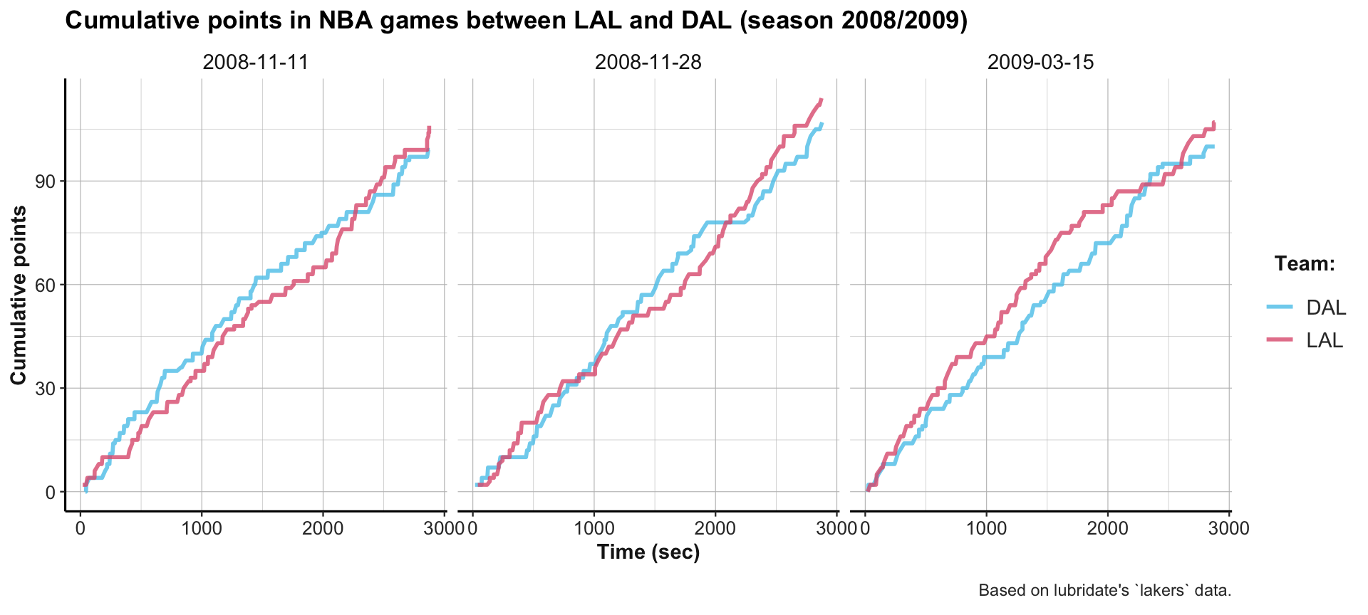
Please note: This dataset and questions like the ones asked here are a good illustration of a possible Data science project. At this point, you should be starting to think about datasets and questions for your own project. (See Appendix C for some guidelines for and the scope of a successful data science projects.)
A.10.6 Exercise 6
DOB and study times
The dataset exp_num_dt (available in the ds4psy package or as a CSV-file from rpository.com) contains the birth dates and study participation times of 1000 ficticious, but surprisingly friendly people.
We read the data file into a tibble dt and select only its date-related variables:
# dt <- readr::read_csv("http://rpository.com/ds4psy/data/dt.csv")  # online
dt <- ds4psy::exp_num_dt  # ds4psy package
# dt

# Select only its date-time related variables:
dt_t <- dt %>% select(name:byear, t_1, t_2)

# Check:
# dt  # 1000 x 7
knitr::kable(head(dt_t), caption = "Time-related variables of table `dt`.")| name | gender | bday | bmonth | byear | t_1 | t_2 |
|---|---|---|---|---|---|---|
| I.G. | male | 14 | 12 | 1968 | 2020-01-16 11:00:58 | 2020-01-16 11:32:21 |
| O.B. | male | 10 | 4 | 1974 | 2020-01-17 14:11:07 | 2020-01-17 15:05:14 |
| M.M. | male | 28 | 9 | 1987 | 2020-01-16 10:06:06 | 2020-01-16 10:51:47 |
| V.J. | female | 15 | 2 | 1978 | 2020-01-10 10:06:04 | 2020-01-10 10:39:48 |
| O.E. | male | 18 | 5 | 1985 | 2020-01-20 09:23:51 | 2020-01-20 10:11:36 |
| Q.W. | male | 1 | 3 | 1968 | 2020-01-13 11:10:09 | 2020-01-13 11:54:07 |
The variables
bday,bmonth, andbyearcontain each participant’s date of birth.- Compute a variable
DOBthat summarizesbday,bmonth, andbyear(in a “Date” variable) and a variablebweekdaythat shows the weekday of each participant’s DOB (as a chacter variable).
- Compute a variable
Hint: A base R solution is about as long as the dplyr/lubridate solution.
Solution
# (a) base R solution:
dt_1 <- dt_t  # copy file
DOB_strings <- paste(dt_1$byear, dt_1$bmonth, dt_1$bday, sep = "-")  # paste DOB string
dt_1$DOB <- as.Date(DOB_strings, format = "%Y-%m-%d")                # parse DOB
dt_1$bweekday <- format(dt_1$DOB, "%a")                              # retrieve weekday
dt_1
#> # A tibble: 1,000 × 9
#>    name  gender  bday bmonth byear t_1                 t_2
#>    <chr> <chr>  <dbl>  <dbl> <dbl> <dttm>              <dttm>
#>  1 I.G.  male      14     12  1968 2020-01-16 11:00:58 2020-01-16 11:32:21
#>  2 O.B.  male      10      4  1974 2020-01-17 14:11:07 2020-01-17 15:05:14
#>  3 M.M.  male      28      9  1987 2020-01-16 10:06:06 2020-01-16 10:51:47
#>  4 V.J.  female    15      2  1978 2020-01-10 10:06:04 2020-01-10 10:39:48
#>  5 O.E.  male      18      5  1985 2020-01-20 09:23:51 2020-01-20 10:11:36
#>  6 Q.W.  male       1      3  1968 2020-01-13 11:10:09 2020-01-13 11:54:07
#>  7 H.K.  male      27      4  1994 2020-01-19 13:54:15 2020-01-19 14:17:26
#>  8 T.R.  female     5      6  1961 2020-01-19 09:38:54 2020-01-19 10:33:33
#>  9 F.J.  male       1     10  1983 2020-01-15 08:24:11 2020-01-15 09:08:13
#> 10 J.R.  female    29     12  1941 2020-01-18 08:54:27 2020-01-18 09:35:21
#> # … with 990 more rows, and 2 more variables: DOB <date>, bweekday <chr>

# (b) lubridate solution:
dt_2 <- dt_t %>%
  mutate(DOB = lubridate::make_date(day = bday, month = bmonth, year = byear),
         bweekday = lubridate::wday(DOB, label = TRUE, abbr = TRUE)) %>%
  select(name:byear, DOB, bweekday, everything()) %>%
  mutate(bweekday = as.character(bweekday))
dt_2
#> # A tibble: 1,000 × 9
#>    name  gender  bday bmonth byear DOB        bweekday t_1
#>    <chr> <chr>  <dbl>  <dbl> <dbl> <date>     <chr>    <dttm>
#>  1 I.G.  male      14     12  1968 1968-12-14 Sat      2020-01-16 11:00:58
#>  2 O.B.  male      10      4  1974 1974-04-10 Wed      2020-01-17 14:11:07
#>  3 M.M.  male      28      9  1987 1987-09-28 Mon      2020-01-16 10:06:06
#>  4 V.J.  female    15      2  1978 1978-02-15 Wed      2020-01-10 10:06:04
#>  5 O.E.  male      18      5  1985 1985-05-18 Sat      2020-01-20 09:23:51
#>  6 Q.W.  male       1      3  1968 1968-03-01 Fri      2020-01-13 11:10:09
#>  7 H.K.  male      27      4  1994 1994-04-27 Wed      2020-01-19 13:54:15
#>  8 T.R.  female     5      6  1961 1961-06-05 Mon      2020-01-19 09:38:54
#>  9 F.J.  male       1     10  1983 1983-10-01 Sat      2020-01-15 08:24:11
#> 10 J.R.  female    29     12  1941 1941-12-29 Mon      2020-01-18 08:54:27
#> # … with 990 more rows, and 1 more variable: t_2 <dttm>

# Verify equality:
all.equal(dt_1$DOB, dt_2$DOB)
#> [1] TRUE
all.equal(dt_1$bweekday, dt_2$bweekday)
#> [1] TRUE
Note: We could also parse DOB as calendar times/date-times (using the as.POSIXct() and make_datetime() functions). However, to obtain identical results in base R and lubridate, we need to specify the same time zone in both solutions (e.g., by setting tz = "").
What would each participant respond to the question
- “How old are you?”
(i.e., what was each person’s age in completed years, when starting the study in January 2020)?
Verify your result for those participants who took part in the study on their birthday.
Hint: This task requires considering both DOB and t_1 (to check whether the person already celebrated his or her birthday in the current year when starting the study at the time t_1).
Solution
dt_2 <- dt_t %>%
  mutate(DOB = lubridate::make_date(day = bday, month = bmonth, year = byear),
         study_date = as.Date(t_1),         # time as date
         year_diff = lubridate::year(t_1) - lubridate::year(DOB),  # difference (in date years)
         life_time = DOB %--% study_date,   # a time interval (between dates)
         life_time_2 = DOB %--% t_1,        # a time interval (between times)
         age = life_time_2 %/% years(1)) %>%  # completed years
  select(name, DOB, t_1, age, year_diff)
dt_2
#> # A tibble: 1,000 × 5
#>    name  DOB        t_1                   age year_diff
#>    <chr> <date>     <dttm>              <dbl>     <dbl>
#>  1 I.G.  1968-12-14 2020-01-16 11:00:58    51        52
#>  2 O.B.  1974-04-10 2020-01-17 14:11:07    45        46
#>  3 M.M.  1987-09-28 2020-01-16 10:06:06    32        33
#>  4 V.J.  1978-02-15 2020-01-10 10:06:04    41        42
#>  5 O.E.  1985-05-18 2020-01-20 09:23:51    34        35
#>  6 Q.W.  1968-03-01 2020-01-13 11:10:09    51        52
#>  7 H.K.  1994-04-27 2020-01-19 13:54:15    25        26
#>  8 T.R.  1961-06-05 2020-01-19 09:38:54    58        59
#>  9 F.J.  1983-10-01 2020-01-15 08:24:11    36        37
#> 10 J.R.  1941-12-29 2020-01-18 08:54:27    78        79
#> # … with 990 more rows

# Check: Participants with bmonth of 1 (January), who may
#        already have celebrated their birthday in 2020:
dt_2 %>% filter(lubridate::month(DOB) == 1)
#> # A tibble: 79 × 5
#>    name  DOB        t_1                   age year_diff
#>    <chr> <date>     <dttm>              <dbl>     <dbl>
#>  1 U.W.  1996-01-12 2020-01-13 10:33:52    24        24
#>  2 U.V.  1990-01-13 2020-01-20 13:00:44    30        30
#>  3 G.H.  1948-01-17 2020-01-17 15:29:00    72        72
#>  4 V.U.  1952-01-22 2020-01-17 11:09:41    67        68
#>  5 T.M.  1994-01-14 2020-01-12 14:45:03    25        26
#>  6 Y.B.  1956-01-10 2020-01-18 15:38:54    64        64
#>  7 H.V.  1973-01-07 2020-01-13 14:28:10    47        47
#>  8 F.H.  1947-01-21 2020-01-19 10:34:42    72        73
#>  9 H.R.  1974-01-14 2020-01-15 13:57:58    46        46
#> 10 R.S.  1972-01-12 2020-01-12 14:20:19    48        48
#> # … with 69 more rows

# Check: Participants starting the study on their birthday:
dt_2 %>%
  filter(lubridate::month(DOB) == lubridate::month(t_1)) %>%
  filter(lubridate::day(DOB) == lubridate::day(t_1))
#> # A tibble: 4 × 5
#>   name  DOB        t_1                   age year_diff
#>   <chr> <date>     <dttm>              <dbl>     <dbl>
#> 1 G.H.  1948-01-17 2020-01-17 15:29:00    72        72
#> 2 R.S.  1972-01-12 2020-01-12 14:20:19    48        48
#> 3 Z.Q.  1992-01-20 2020-01-20 09:08:33    28        28
#> 4 N.Z.  1994-01-13 2020-01-13 10:08:16    26        26
The time variables
t_1andt_2indicate the start and end times of each person’s participation in this study.- Compute the duration of each person’s participation (in minutes and seconds) and plot the distribution of the resulting durations (e.g., as a histogram).
Solution
dt_3 <- dt %>%
  mutate(t_diff = (t_2 - t_1),
         dur = as.duration(t_2 - t_1))
# dt_3

# Get means:
dur_mn <- mean(dt_3$dur)    # mean
dur_md <- median(dt_3$dur)  # median

# Plot histograms:

## base R:
# hist(as.numeric(dt$dur), breaks = 20, col = unikn::Seeblau)

# ggplot:
ggplot(dt_3, aes(x = as.numeric(dur))) +
  geom_histogram(col = "black", binwidth = 200, fill = unikn::Seeblau) +
  geom_vline(xintercept = dur_mn, col = "gold", linetype = 1, size = 1) +
  geom_vline(xintercept = dur_md, col = unikn::Pinky, linetype = 2, size = 1) +
  labs(title = "Distribution of durations", x = "Duration (in seconds)") +
  ds4psy::theme_ds4psy()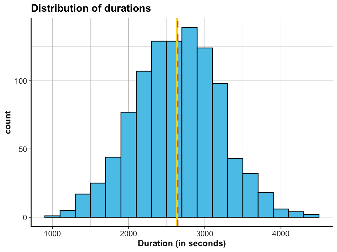
The study officially only ran for 5 days — from “2020-01-13” to “2020-01-18” — and should only include participants that responded in up to one hour (60 minutes).
- Add a filter variable
validthat enforces these criteria (i.e., allows filtering out participants with other dates and durations longer than 60 minutes).
- Add a filter variable
Solution
dt_4 <- dt_3 %>%
  mutate(date = as_date(t_1),
         valid_date = (date >= "2020-01-13") & (date <= "2020-01-18"),
         valid_dur  = (dur <= as.duration(60 * 60)),
         valid      = valid_date & valid_dur) %>%
  filter(valid)

# Filtered data:
dt_4
#> # A tibble: 519 × 21
#>    name  gender  bday bmonth byear height blood_type bnt_1 bnt_2 bnt_3 bnt_4
#>    <chr> <chr>  <dbl>  <dbl> <dbl>  <dbl> <chr>      <dbl> <dbl> <dbl> <dbl>
#>  1 I.G.  male      14     12  1968    169 O+             1     0     0     1
#>  2 O.B.  male      10      4  1974    181 O+             1     1     1    NA
#>  3 M.M.  male      28      9  1987    183 A-             0     1     0     0
#>  4 Q.W.  male       1      3  1968    172 A+             1     1     1     0
#>  5 F.J.  male       1     10  1983    158 O+             0     0     0     0
#>  6 J.R.  female    29     12  1941    157 O+             1     1     0     1
#>  7 K.E.  male      10     12  1951    161 A+             0     0     1     1
#>  8 U.W.  female    12      1  1996    161 O+             0     1     0     0
#>  9 J.Y.  female    20      5  1987    155 O-             0     1     1    NA
#> 10 S.X.  female     5      3  1986    169 O+             1     0     0     1
#> # … with 509 more rows, and 10 more variables: g_iq <dbl>, s_iq <dbl>,
#> #   t_1 <dttm>, t_2 <dttm>, t_diff <drtn>, dur <Duration>, date <date>,
#> #   valid_date <lgl>, valid_dur <lgl>, valid <lgl>

# Check: Does the filter work as intended?
min(dt_4$t_1)
#> [1] "2020-01-13 08:09:30 UTC"
max(dt_4$t_1)
#> [1] "2020-01-18 17:50:53 UTC"
max(dt_4$dur)
#> [1] 3600
Finally, we can compute some basic descriptives of the participants considered to be
valid:- How many participants remain in the sample of valid data?
- What is their average
heightandg_iqscore?
- How many participants remain in the sample of valid data?
Solution
# Get descriptives (by hand):
nrow(dt_4)  # N of valid participants
#> [1] 519
mean(dt_4$height)
#> [1] 166.2852
mean(dt_4$g_iq, na.rm = TRUE)  # There are NA values!
#> [1] 101.5207
sum(!is.na(dt_4$g_iq))         # N of non-NA values?
#> [1] 507

# All in one dplyr pipe:
dt_4 %>%
  summarise(N = n(),
            mn_height = mean(height),
            N_hg_nonNA = sum(!is.na(height)),
            mn_iq = mean(g_iq, na.rm = TRUE),
            N_iq_nonNA = sum(!is.na(g_iq)))
#> # A tibble: 1 × 5
#>       N mn_height N_hg_nonNA mn_iq N_iq_nonNA
#>   <int>     <dbl>      <int> <dbl>      <int>
#> 1   519      166.        519  102.        507
A.10.7 Exercise 7
Bonus task: Evaluating time differences
This exercise creates random time differences and compares the results of computing them in two different ways.
Use the
sample_time()function of ds4psy to generate vectors ofNrandom starting times andNrandom end times.Compute and compare the time difference between both vectors for various units of time. Specifically, compare the solutions of the
diff_times()function of ds4psy with the corresponding lubridate solution (using time intervals and periods).Continue comparing the results of both solution methods until you find some examples with different solutions for the same time difference. Can you explain the discrepancies?
Hint: Here is a possible setup for an investigation of this type:
# Parameters:
N <- 10
t1 <- "2020-01-01 00:00:00"
t2 <- Sys.time()

# Random time vectors:
t_start <- ds4psy::sample_time(from = t1, to = t2, size = N)
t_end   <- ds4psy::sample_time(from = t1, to = t2, size = N)

# in months:
ds4psy::diff_times(t_start, t_end, unit = "months", as_character = FALSE)
lubridate::as.period(lubridate::interval(t_start, t_end), unit = "months")

# in days:
ds4psy::diff_times(t_start, t_end, unit = "days", as_character = FALSE)
lubridate::as.period(lubridate::interval(t_start, t_end), unit = "days")
Solution
Here are some examples with discrepancies between solutions (different day counts):
# (1)
t1 <- "2020-04-14 10:00:00"
t2 <- "2020-02-25 05:00:00"

ds4psy::diff_times(t1, t2, unit = "months", as_character = TRUE)
#> [1] "-1m 20d 5H 0M 0S"
lubridate::as.period(lubridate::interval(t1, t2), unit = "months")
#> [1] "-1m -18d -5H 0M 0S"

# (2)
t1 <- "2020-05-11 12:00:00"
t2 <- "2020-02-15 10:00:00"

ds4psy::diff_times(t1, t2, unit = "months", as_character = TRUE)
#> [1] "-2m 26d 2H 0M 0S"
lubridate::as.period(lubridate::interval(t1, t2), unit = "months")
#> [1] "-2m -25d -2H 0M 0S"

# (3)
t1 <- "2020-03-15 15:00:00"
t2 <- "2020-01-28 16:00:00"

ds4psy::diff_times(t1, t2, unit = "months", as_character = TRUE)
#> [1] "-1m 15d 23H 0M 0S"
lubridate::as.period(lubridate::interval(t1, t2), unit = "months")
#> [1] "-1m -17d -23H 0M 0S"
Answer: Negative time intervals are occasionally handled differently by both packages.
In ds4psy, the solution of diff_times(t1, t2) is the negation of diff_times(t2, t1), which corresponds to our understanding of subtraction.
This concludes our exercises on creating and computing with dates and times.