A.12 Solutions (12)

Here are the solutions to the basic exercises on loops and applying functions to data structures of Chapter 12 (Section 12.5).
A.12.1 Exercise 1
Fibonacci loop and functions
- Look up the term Fibonacci numbers (e.g., on Wikipedia) and use a
forloop to create a numeric vector of the first 25 Fibonacci numbers (for a series of numbers starting with0, 1).
Hint: The series of Fibonacci numbers was previously introduced in our discussion of recursion (see Section 11.4.1). We are now looking for an iterative definition, but the underlying processes are quite similar. Essentially, the recursive definition resulted in an implicit loop, whereas we now explicitly define the iteration.
Incorporate your
forloop into afibonaccifunction that returns a numeric vector of the firstnFibonacci numbers. Test your function forfibonacci(n = 25).Generalize your
fibonaccifunction to also accept the first two elements (e1ande2) as inputs to the series and then create the firstnFibonacci numbers given these initial elements. Test your function forfibonacci(e1 = 1, e2 = 3, n = 25).
Solution
- According to Wikipedia, a Fibonacci sequence is the integer sequence of
0, 1, 1, 2, 3, 5, 8, ....
Thus, the first 2 elements \(e_{1}\) and \(e_{2}\) of the series need to be provided. For \(i > 2\), each element \(e_{i}\) is the sum of the two preceding elements:
\(e_{i} = e_{i-2} + e_{i-1}\).
We turn this into a for loop as follows:
# 1: Loop to print 25 Fibonacci numbers
N <- 25             # length of series
fib <- rep(NA, 25)  # prepare output

for (i in 1:N){

  # Distinguish between 3 cases:
  if (i==1) { fib[i] <- 0 }  # initialize 1st element
  if (i==2) { fib[i] <- 1 }  # initialise 2nd element

  if (i > 2) {
    fib[i] <- fib[i-2] + fib[i-1]
  }

}

# Result:
fib
#>  [1]     0     1     1     2     3     5     8    13    21    34    55    89
#> [13]   144   233   377   610   987  1597  2584  4181  6765 10946 17711 28657
#> [25] 46368- Incorporating the
forloop into a functionfibonacci(n):
fibonacci <- function(n){

  if (is.na(n) || (n < 1) || (n != round(n)))  {
    stop("n must be a positive integer.")
  }

  fib <- rep(NA, n)  # initialize output vector

  for (i in 1:n){

    # Distinguish between 3 cases:
    if (i==1) { fib[i] <- 0 }  # initialize 1st element
    if (i==2) { fib[i] <- 1 }  # initialise 2nd element

    if (i > 2) {
      fib[i] <- fib[i-2] + fib[i-1]
    }

  }

  return(fib)

}
Checking the function:
# Check:
fibonacci(1)
#> [1] 0
fibonacci(2)
#> [1] 0 1
fibonacci(3)
#> [1] 0 1 1
fibonacci(4)
#> [1] 0 1 1 2

# First 25 Fibonacci numbers:
fibonacci(25)
#>  [1]     0     1     1     2     3     5     8    13    21    34    55    89
#> [13]   144   233   377   610   987  1597  2584  4181  6765 10946 17711 28657
#> [25] 46368

## Errors:
# fibonacci(0)
# fibonacci(-1)
# fibonacci(3/2)
# fibonacci(NA)
Realizing that we only need the for loop when n > 2, we could re-write the same function as follows:
fibonacci <- function(n){

  if (is.na(n) || (n < 1) || (n != round(n)))  {
    stop("n must be a positive integer.")
  }

  # initialize the 1st and 2nd elements:
  fib <- c(0, 1)

  if (n <= 2){

    fib <- fib[1:n]

  } else {

    # initialize output vector:
    fib <- c(fib, rep(NA, (n-2)))

    # loop:
    for (i in 3:n){

      fib[i] <- fib[i-2] + fib[i-1]

    } # end for loop.
  } # end if (n > 2).

  return(fib)

}
Checking the function:
# Check:
fibonacci(1)
#> [1] 0
fibonacci(2)
#> [1] 0 1
fibonacci(3)
#> [1] 0 1 1
fibonacci(4)
#> [1] 0 1 1 2

# First 25 Fibonacci numbers:
fibonacci(25)
#>  [1]     0     1     1     2     3     5     8    13    21    34    55    89
#> [13]   144   233   377   610   987  1597  2584  4181  6765 10946 17711 28657
#> [25] 46368

## Errors:
# fibonacci(0)
# fibonacci(-1)
# fibonacci(3/2)
# fibonacci(NA)- Generalizing
fibonacci(n)to a functionfibonacci(e1, e2, n)is simple: The following version makes the argumentse1ande2optional to return the standard sequence by default.
fibonacci <- function(e1 = 0, e2 = 1, n){

  if (is.na(n) || (n < 1) || (n != round(n)))  {
    stop("n must be a positive integer.")
  }

  fib <- rep(NA, n)  # initialize output vector

  for (i in 1:n){

    # Distinguish between 3 cases:
    if (i==1) { fib[i] <- e1 }  # initialize 1st element
    if (i==2) { fib[i] <- e2 }  # initialise 2nd element

    if (i > 2) {
      fib[i] <- fib[i-2] + fib[i-1]
    }

  }

  return(fib)

}
This generalized fibonacci function still allows all previous calls, like:
fibonacci(n = 25)
#>  [1]     0     1     1     2     3     5     8    13    21    34    55    89
#> [13]   144   233   377   610   987  1597  2584  4181  6765 10946 17711 28657
#> [25] 46368
but now also allows specifying different initial elements:
fibonacci(e1 = 1, e2 = 3, n = 25)
#>  [1]      1      3      4      7     11     18     29     47     76    123
#> [11]    199    322    521    843   1364   2207   3571   5778   9349  15127
#> [21]  24476  39603  64079 103682 167761
A.12.2 Exercise 2
Looping for divisors
- Write a
forloop that prints out all positive divisors of the number 1000.
Hint: Use N %% x == 0 to test whether x is a divisor of N.
Solution
N <- 1000

for (i in 1:N){

  if (N %% i == 0)
    print(i)

}
#> [1] 1
#> [1] 2
#> [1] 4
#> [1] 5
#> [1] 8
#> [1] 10
#> [1] 20
#> [1] 25
#> [1] 40
#> [1] 50
#> [1] 100
#> [1] 125
#> [1] 200
#> [1] 250
#> [1] 500
#> [1] 1000- How many iterations did your loop require? Could you achieve the same results with fewer iterations?
Solution
Our first for loop required N = 1000 iterations.
However, we could use the insight that finding any divisor actually yields two solutions — a divisor \(x\) and its complement \(y = N/x\).
This allows limiting our search to a range from 1 to a maximum of \(\sqrt{N}\):
# Using a maximum of sqrt(N) loops:
N <- 1000

seq <- c(1:floor(sqrt(N)))  # seq of max. length sqrt(N)
# seq

length(seq)
#> [1] 31

for (i in seq){

  if (N %% i == 0)
    print(paste0(i, " x ", N/i))

}
#> [1] "1 x 1000"
#> [1] "2 x 500"
#> [1] "4 x 250"
#> [1] "5 x 200"
#> [1] "8 x 125"
#> [1] "10 x 100"
#> [1] "20 x 50"
#> [1] "25 x 40"- Write a
divisorsfunction that uses aforloop to return a numeric vector containing all positive divisors of a natural numberN.
Hint: Note that we do not know the length of the resulting vector.
Solution
divisors <- function(N){

  # check inputs:
  if ( is.na(N) || (N < 1) || (N %% 1 != 0)) { stop("N should be a natural number.") }

  # initialize:
  seq <- c(1:floor(sqrt(N)))  # seq of max. length sqrt(N)
  out <- c()  # prepare output vector

  # loop:
  for (i in seq){

    if (N %% i == 0) {  # i is a divisor of N:
      out <- c(out, i, N/i)  # add i and N/i to out
    }

  } # end loop.

  # Remove duplicates and sort output:
  out <- sort(unique(out))

  return(out)

}

# Check:
divisors(1)
#> [1] 1
divisors(8)
#> [1] 1 2 4 8
divisors(9)
#> [1] 1 3 9
divisors(12)
#> [1]  1  2  3  4  6 12
divisors(13)
#> [1]  1 13

# Note errors for:
# divisors(NA)
# divisors(-10)
# divisors(1/2)- Use your
divisorsfunction to answer the question: Does the number 1001 have fewer or more divisors than the number 1000?
(d_1000 <- divisors(1000))
#>  [1]    1    2    4    5    8   10   20   25   40   50  100  125  200  250  500
#> [16] 1000

(d_1001 <- divisors(1001))
#> [1]    1    7   11   13   77   91  143 1001

# 1000 has more divisors than 1001:
length(d_1000) > length(d_1001)
#> [1] TRUE- Use your
divisorsfunction and anotherforloop to answer the question: Which prime numbers exist between the number 111 and the number 1111?
Hint: A prime number (e.g., 13) has only two divisors: 1 and the number itself.
# Parameters:
range_min <- 111
range_max <- 1111
primes_found <- c()  # initialize

for (i in range_min:range_max) {

  if (length(divisors(i)) == 2){

    primes_found <- c(primes_found, i)

  }

}

# Solution:
primes_found
#>  [1] 113 127 131 137 139 149 151 157 163 167 173 179 181 191 193 197 199 211 223
#> [20] 227 229 233 239 241 251 257 263 269 271 277 281 283 293 307 311 313 317 331
#> [39] 337 347 349 353 359 367 373 379 383 389 397 401 409 419 421 431 433 439 443
#> [58] 449 457 461 463 467 479 487 491 499 503 509 521 523 541 547 557 563 569
#>  [ reached getOption("max.print") -- omitted 82 entries ]
length(primes_found)
#> [1] 157
Note some details:
The loop above uses the
divisorsfunction within aforloop (in the rangerange_min:range_max). As thedivisorsfunction also uses aforloop to find all divisors ofN, we are using a loop inside a loop. As such structures can quickly become very inefficient, it is a good idea to try reducing the number of iterations when possible.The condition
length(divisors(i)) == 2would fail to detect the prime number \(N = 1\). A more general solution would first define anis_prime()function and then useis_prime(N)in theifstatement of theforloop:
is_prime <- function(N){

  if ( is.na(N) || (N < 1) || (N %% 1 != 0)) { stop("N should be a natural number.") }

  out <- NA  # initialize

  if (N == 1) {

    out <- TRUE  # 1 is a prime number

  } else {

    if (length(divisors(N)) == 2) {
      out <- TRUE
    } else {
      out <- FALSE
    }

  }

  return(out)

}

# Check:
is_prime(1)
#> [1] TRUE
is_prime(101)
#> [1] TRUE

is_prime(111)
#> [1] FALSE
divisors(111)
#> [1]   1   3  37 111

# Errors for:
# is_prime(NA)
# is_prime(0)
# is_prime(3/2)
The is_prime() function can be written in many different ways, of course.
Check out this stackoverflow thread for solutions.
A.12.3 Exercise 3
Let’s revisit our favorite randomizing devices one more time:
In Chapter 1, we first explored the ds4psy functions
coin()anddice()(see Section 1.6.4 and Exercise 3 in Section 1.8.3).In Exercise 4 of Chapter 11 (see Section 11.6.4), we wrote
my_coin()andmy_dice()functions by calling either these ds4psy functions or the base Rsample()function.In this exercise, we will use
forandwhileloops to repeatedly call an existing function.
Throwing dice in loops
- Implement a function
my_dicethat uses the base R functionsample()to simulate a throw of a dice (i.e., yielding an integer from 1 to 6 with equal probability).
Solution
my_dice <- function() {
  sample(x = 1:6, size = 1)
}

# Check:
my_dice()
#> [1] 5
# Using for loop to throw dice 10 times:
for (i in 1:10){
  print(my_dice())
}
#> [1] 2
#> [1] 5
#> [1] 4
#> [1] 5
#> [1] 5
#> [1] 5
#> [1] 1
#> [1] 1
#> [1] 6
#> [1] 2- Add an argument
N(for the number of throws) to your function and modify it by using aforloop to throw the diceNtimes, and returning a vector of lengthNthat shows the results of theNthrows.
Hint: This task corresponds to Exercise 4 of Chapter 11 (see Section 11.6.4).
Solution
my_dice <- function(N = 1) {

  out <- rep(NA, N)

  for (i in 1:N){

    out[i] <- sample(x = 1:6, size = 1)

  } # end for loop.

  return(out)

}

# Check:
my_dice()
#> [1] 1
my_dice(10)  # throw dice 10 times
#>  [1] 4 6 4 3 6 2 3 5 3 6
Note: As the sample function contains a size argument, a simpler version of the same function could have been:
my_dice <- function(N = 1) {
  sample(x = 1:6, size = N, replace = TRUE)
}

# Check:
my_dice()
#> [1] 5
my_dice(10)  # throw dice 10 times
#> [1] 6 2 4 1 3 6 4 1 2 5- Use a
whileloop to throwmy_dice(N = 1)until you throw the number 6 twice in a row and show the sequence of all throws up to this point.
Hint: Given a sequence throws, the i-th element is throws[i].
Hence, the last element of throws is throws[length(throws)].
Solution
throws <- c(my_dice(1), my_dice(1))  # first 2 throws
throws
#> [1] 2 1

while (!( (throws[length(throws) - 1] == 6) &&
          (throws[length(throws)] == 6) )) {

          throws <- c(throws, my_dice(1))  # throw dice(1) and add it to throws

}

throws
#> [1] 2 1 1 1 1 5 2 6 5 3 2 4 6 1 3 4 4 2 1 4 6 1 5 2 5 2 2 6 6- Use your solution of 3. to conduct a simulation that addresses the following question:
- How many times on average do we need to throw
my_dice(1)to obtain the number 6 twice in a row?
Hint: Use a for loop to run your solution to 3. for T = 10000 times and store the length of the individual throws in a numeric vector.
Solution
T <- 10000

out <- rep(NA, T)  # initialize output vector

for (n in 1:T){

  throws <- c(my_dice(1), my_dice(1))  # first 2 throws

  while (!( (throws[length(throws) - 1] == 6) &&
            (throws[length(throws)] == 6) )) {

    throws <- c(throws, my_dice(1))  # throw dice(1) and add it to throws
  }

  out[n] <- length(throws)

}

# Results:
summary(out)
#>    Min. 1st Qu.  Median    Mean 3rd Qu.    Max.
#>    2.00   13.00   30.00   41.89   58.00  380.00
A histogram shows the distribution of the number of throws needed:
library(tidyverse)
library(unikn)

# Turn out into a tibble:
tb <- tibble(nr = out)
# tb

# Define labels:
cp_lbl <- paste0("(Simulation of T = ", T, " trials)")
mn_lbl <- paste0("mean = ", round(mean(out), 2))
md_lbl <- paste0("median = ", round(median(out), 2))

# Histogram of individual number of throws:
ggplot(tb) +
  geom_histogram(aes(x = nr), binwidth = 5, fill = Seeblau, color = "white") +
  coord_cartesian(xlim = c(0, 200)) +  # do not show values beyond x = 200
  # Show mean and median:
  geom_vline(xintercept = mean(out), linetype = 1, color = Bordeaux) +  # mean line
  annotate("text", label = mn_lbl, x = mean(out) + 20, y = 950, color = Bordeaux) +
  geom_vline(xintercept = median(out), linetype = 2, color = Karpfenblau) +  # median line
  annotate("text", label = md_lbl, x = median(out) + 18, y = 750, color = Karpfenblau) +
  # Text and formatting:
  labs(title = "Number of throws needed to get 6 twice in a row",
       x = "N", y = "Frequency", caption = cp_lbl) +
  ds4psy::theme_ds4psy(col_title = "black")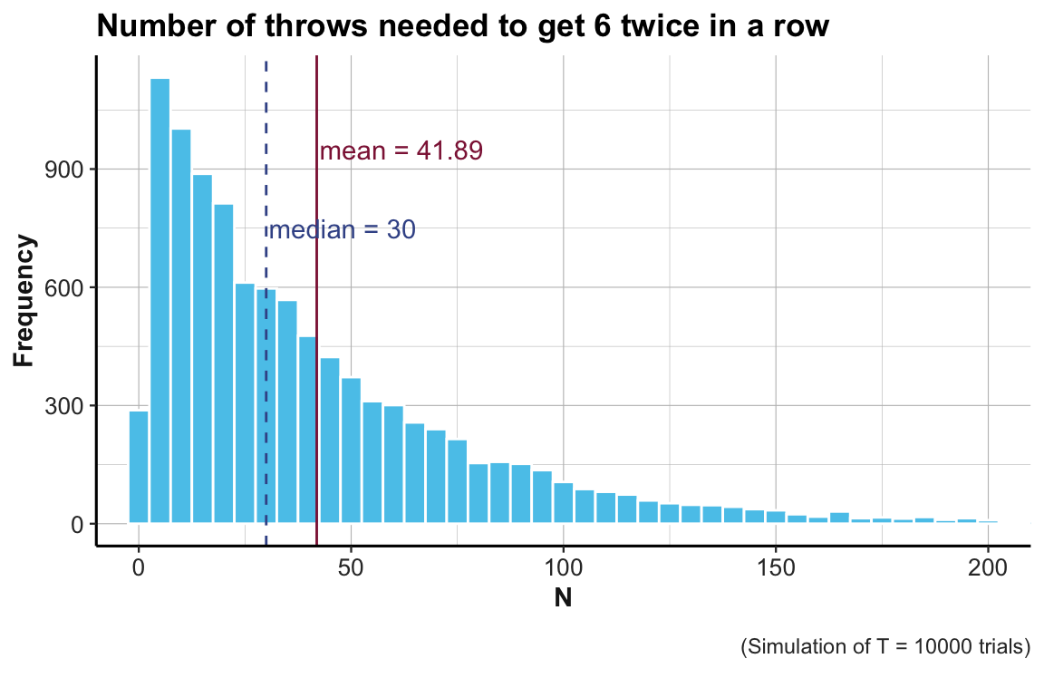
Disclaimer
This exercise shows how loops can be used to generate and collect multiple outputs. This can sometimes replace vector arguments to functions. However, as R is optimized for vectors, using loops rather than vectors is not generally recommended.
A.12.4 Exercise 4
Mapping functions to data
Write code that uses a function of the base R apply or purrr map family of functions to:
- Compute the mean of every column in
mtcars.
- Determine the type of each column in
ggplot2::diamonds.
- Compute the number of unique values in each column of
iris.
- Generate 10 random normal numbers for each of
μ = −100, 0, and 100.
Note: This exercise is based on Exercise 1 of Chapter 21.5.3 in r4ds.
Solution
# 1. Compute the mean of every column in `mtcars`:

# (a) Solve for 1st column:
mean(mtcars$mpg)
#> [1] 20.09062

# (b) Generalize to all columns:
as_tibble(mtcars) %>% map_dbl(mean)
#>        mpg        cyl       disp         hp       drat         wt       qsec
#>  20.090625   6.187500 230.721875 146.687500   3.596563   3.217250  17.848750
#>         vs         am       gear       carb
#>   0.437500   0.406250   3.687500   2.812500
apply(X = mtcars, MARGIN = 2, FUN = mean)
#>        mpg        cyl       disp         hp       drat         wt       qsec
#>  20.090625   6.187500 230.721875 146.687500   3.596563   3.217250  17.848750
#>         vs         am       gear       carb
#>   0.437500   0.406250   3.687500   2.812500

# 2. Determine the type of each column in `ggplot2::diamonds`:

# (a) Solve for 1st column:
typeof(ggplot2::diamonds$carat)  # solution for 1st column
#> [1] "double"

# (b) Generalize to all columns:
ggplot2::diamonds %>% map_chr(typeof)
#>     carat       cut     color   clarity     depth     table     price         x
#>  "double" "integer" "integer" "integer"  "double"  "double" "integer"  "double"
#>         y         z
#>  "double"  "double"
apply(X = ggplot2::diamonds, MARGIN = 2, FUN = typeof)
#>       carat         cut       color     clarity       depth       table
#> "character" "character" "character" "character" "character" "character"
#>       price           x           y           z
#> "character" "character" "character" "character"
# Note: All variables viewed as characters!

# 3. Compute the number of unique values in each column of `iris`:

# (a) Solve for 1st column:
n_distinct(iris$Sepal.Length)  # solution for 1st column
#> [1] 35

# (b) Generalize to all columns:
as_tibble(iris) %>% map_int(n_distinct)
#> Sepal.Length  Sepal.Width Petal.Length  Petal.Width      Species
#>           35           23           43           22            3
apply(X = iris, MARGIN = 2, FUN = n_distinct)
#> Sepal.Length  Sepal.Width Petal.Length  Petal.Width      Species
#>           35           23           43           22            3

# 4. Generate 10 random normal numbers for each of `μ = −100, 0, and 100`:

# (a) Solve for 1st mean:
mu <- c(-100, 0, 100)
rnorm(n = 10, mean = mu[1])
#>  [1]  -99.47997 -100.56539  -99.73644  -99.55538 -100.85245 -100.77212
#>  [7]  -99.84320  -98.49620  -99.81847  -98.80089

# (b) Generalize to all means:
mu %>% map(rnorm, n = 10) %>% str()
#> List of 3
#>  $ : num [1:10] -99.5 -99.4 -101.4 -99 -99.8 ...
#>  $ : num [1:10] -0.7202 0.1053 -0.0766 0.0753 0.1168 ...
#>  $ : num [1:10] 101 100 99.2 98.5 101.7 ...
lapply(X = mu, FUN = rnorm, n = 10) %>% str()
#> List of 3
#>  $ : num [1:10] -99.9 -99.2 -99 -100.4 -98.7 ...
#>  $ : num [1:10] 0.851 0.452 0.833 0.837 -1.4 ...
#>  $ : num [1:10] 101 101 100 101 101 ...

# Note: In 4(b), we add str() to show the structure of the output lists.
A.12.5 Exercise 5
Z-transforming tables
In this exercise, we will standardize an entire table of data (using a for loop, an apply, and a map function).
We will first write a utility function that achieves the desired transformation for a vector and then compare and contrast different ways of applying this function to a table of data.
In case you are not familiar with the notion of a z score or standard score, look up these terms (e.g., on Wikipedia).
- Write a function called
z_transthat takes a vectorvas input and returns the z-transformed (or standardized) values as output ifvis numeric and returnsvunchanged if it is non-numeric.
Hint: Remember that z <- (v - mean(v)) / sd(v)), but beware that v could contain NA values.
Solution
z_trans <- function(v) {

    if (!is.numeric(v)) {
      message("z_trans: v is not numeric: Leaving as is...")
      return(v)
    }

    if (NA %in% v) {
      warning("z_trans: v contains NA-values (ignored here).")
    }

    result <- (v - mean(v, na.rm = TRUE)) / sd(v, na.rm = TRUE)

    return(result)
}

# Check:
z_trans(v = c(-10:10))
#>  [1] -1.6116459 -1.4504813 -1.2893167 -1.1281521 -0.9669876 -0.8058230
#>  [7] -0.6446584 -0.4834938 -0.3223292 -0.1611646  0.0000000  0.1611646
#> [13]  0.3223292  0.4834938  0.6446584  0.8058230  0.9669876  1.1281521
#> [19]  1.2893167  1.4504813  1.6116459
z_trans(v = letters[1:5])
#> [1] "a" "b" "c" "d" "e"
z_trans(v = (1:4 > 2))
#> [1] FALSE FALSE  TRUE  TRUE

## Check messages:
# z_trans(v = c("A", "B"))
# z_trans(v = c(-1, NA, 1))- Load the dataset for the false positive psychology (see Section B.2 of Appendix B) into
falsePosPsyand remove any non-numeric variables from it.
# Load data:
falsePosPsy <- ds4psy::falsePosPsy_all  # from ds4psy package
# falsePosPsy <- readr::read_csv("http://rpository.com/ds4psy/data/falsePosPsy_all.csv")  # online

falsePosPsy
#> # A tibble: 78 × 19
#>    study    ID  aged aged365 female   dad   mom potato when64 kalimba cond
#>    <dbl> <dbl> <dbl>   <dbl>  <dbl> <dbl> <dbl>  <dbl>  <dbl>   <dbl> <chr>
#>  1     1     1  6765    18.5      0    49    45      0      0       1 control
#>  2     1     2  7715    21.1      1    63    62      0      1       0 64
#>  3     1     3  7630    20.9      0    61    59      0      1       0 64
#>  4     1     4  7543    20.7      0    54    51      0      0       1 control
#>  5     1     5  7849    21.5      0    47    43      0      1       0 64
#>  6     1     6  7581    20.8      1    49    50      0      1       0 64
#>  7     1     7  7534    20.6      1    56    55      0      0       1 control
#>  8     1     8  6678    18.3      1    45    45      0      1       0 64
#>  9     1     9  6970    19.1      0    53    51      1      0       0 potato
#> 10     1    10  7681    21.0      0    53    51      0      1       0 64
#> # … with 68 more rows, and 8 more variables: root <dbl>, bird <dbl>,
#> #   political <dbl>, quarterback <dbl>, olddays <dbl>, feelold <dbl>,
#> # computer <dbl>, diner <dbl>- Use an appropriate
mapfunction to to create a single vector that — for each column infalsePosPsy— indicates whether or not it is a numeric variable?
Hint: The function is.numeric tests whether a vector is numeric.
Solution
# (a) Solve for individual variables:
is.numeric(falsePosPsy$kalimba)
#> [1] TRUE
is.numeric(falsePosPsy$cond)
#> [1] FALSE

# (b) Generalize to entire table:
numeric_cols <- falsePosPsy %>% map_lgl(is.numeric)
numeric_cols
#>       study          ID        aged     aged365      female         dad
#>        TRUE        TRUE        TRUE        TRUE        TRUE        TRUE
#>         mom      potato      when64     kalimba        cond        root
#>        TRUE        TRUE        TRUE        TRUE       FALSE        TRUE
#>        bird   political quarterback     olddays     feelold    computer
#>        TRUE        TRUE        TRUE        TRUE        TRUE        TRUE
#>       diner
#> TRUE- Use this vector to select only the numeric columns of
falsePosPsyinto a new tibblefpp_numeric:
Solution
# Indexing columns of falsePosPsy by numeric_cols:
fpp_numeric <- falsePosPsy[ , numeric_cols]
# fpp_numeric

# Alternative solution:
fpp_numeric_1 <- falsePosPsy[, map_lgl(falsePosPsy, is.numeric)]
all.equal(fpp_numeric, fpp_numeric_1)
#> [1] TRUE

# Using dplyr::select:
fpp_numeric_2 <- falsePosPsy %>% dplyr::select(-cond)  # notice that `cond` is non-numeric
all.equal(fpp_numeric, fpp_numeric_2)
#> [1] TRUE- Use a
forloop to apply yourz_transfunction tofpp_numericto standardize all of its columns:
Solution
out <- c()  # prepare output vector

# for loop:
for (i in seq_along(fpp_numeric)){

  out <- cbind(out, z_trans(fpp_numeric[[i]]))

}

# Result:
# out- Turn your resulting data structure into a tibble
out_1and print it.
Solution
# Print result (as tibble):
out_1 <- as_tibble(out)
out_1
#> # A tibble: 78 × 18
#>        V1    V2      V3      V4     V5      V6      V7     V8     V9    V10
#>     <dbl> <dbl>   <dbl>   <dbl>  <dbl>   <dbl>   <dbl>  <dbl>  <dbl>  <dbl>
#>  1 -0.873 -1.70 -0.902  -0.902  -0.873 -0.756  -1.13   -0.807 -0.682  1.59
#>  2 -0.873 -1.65  0.128   0.128   1.13   2.02    2.11   -0.807  1.45  -0.623
#>  3 -0.873 -1.61  0.0362  0.0362 -0.873  1.63    1.54   -0.807  1.45  -0.623
#>  4 -0.873 -1.57 -0.0582 -0.0582 -0.873  0.237   0.0171 -0.807 -0.682  1.59
#>  5 -0.873 -1.52  0.274   0.274  -0.873 -1.15   -1.51   -0.807  1.45  -0.623
#>  6 -0.873 -1.48 -0.0170 -0.0170  1.13  -0.756  -0.173  -0.807  1.45  -0.623
#>  7 -0.873 -1.43 -0.0680 -0.0680  1.13   0.634   0.779  -0.807 -0.682  1.59
#>  8 -0.873 -1.39 -0.996  -0.996   1.13  -1.55   -1.13   -0.807  1.45  -0.623
#>  9 -0.873 -1.35 -0.680  -0.680  -0.873  0.0382  0.0171  1.22  -0.682 -0.623
#> 10 -0.873 -1.30  0.0915  0.0915 -0.873  0.0382  0.0171 -0.807  1.45  -0.623
#> # … with 68 more rows, and 8 more variables: V11 <dbl>, V12 <dbl>, V13 <dbl>,
#> #   V14 <dbl>, V15 <dbl>, V16 <dbl>, V17 <dbl>, V18 <dbl>
Note that we use cbind rather than c within the for loop to add the results of z_trans to out.
This is because z_trans returns a vector for every column of only_numeric.
Alternatively, we also could have constructed a very long vector (with a length of nrow(fpp_numeric) x ncol(fpp_numeric) = 78 x 18 = 1404) and turned it into a rectangular table later.
- Repeat the task of 2. (i.e., applying
z_transto all numeric columns offalsePosPsy) by using the base Rapplyfunction, rather than aforloop. Save and print your resulting data structure as a tibbleout_2.
Hint: Remember to set the MARGIN argument to apply z_trans over all columns, rather than rows.
Solution
# Data:
# fpp_numeric

out_2 <- apply(X = fpp_numeric, MARGIN = 2, FUN = z_trans)

# Print result (as tibble):
out_2 <- as_tibble(out_2)
out_2
#> # A tibble: 78 × 18
#>     study    ID    aged aged365 female     dad     mom potato when64 kalimba
#>     <dbl> <dbl>   <dbl>   <dbl>  <dbl>   <dbl>   <dbl>  <dbl>  <dbl>   <dbl>
#>  1 -0.873 -1.70 -0.902  -0.902  -0.873 -0.756  -1.13   -0.807 -0.682   1.59
#>  2 -0.873 -1.65  0.128   0.128   1.13   2.02    2.11   -0.807  1.45   -0.623
#>  3 -0.873 -1.61  0.0362  0.0362 -0.873  1.63    1.54   -0.807  1.45   -0.623
#>  4 -0.873 -1.57 -0.0582 -0.0582 -0.873  0.237   0.0171 -0.807 -0.682   1.59
#>  5 -0.873 -1.52  0.274   0.274  -0.873 -1.15   -1.51   -0.807  1.45   -0.623
#>  6 -0.873 -1.48 -0.0170 -0.0170  1.13  -0.756  -0.173  -0.807  1.45   -0.623
#>  7 -0.873 -1.43 -0.0680 -0.0680  1.13   0.634   0.779  -0.807 -0.682   1.59
#>  8 -0.873 -1.39 -0.996  -0.996   1.13  -1.55   -1.13   -0.807  1.45   -0.623
#>  9 -0.873 -1.35 -0.680  -0.680  -0.873  0.0382  0.0171  1.22  -0.682  -0.623
#> 10 -0.873 -1.30  0.0915  0.0915 -0.873  0.0382  0.0171 -0.807  1.45   -0.623
#> # … with 68 more rows, and 8 more variables: root <dbl>, bird <dbl>,
#> #   political <dbl>, quarterback <dbl>, olddays <dbl>, feelold <dbl>,
#> # computer <dbl>, diner <dbl>- Repeat the task of 2. and 3. (i.e., applying
z_transto all numeric columns offalsePosPsy) by using an appropriate version of amapfunction from the purrr package. Save and print your resulting data structure as a tibbleout_3.
Hint: Note that the desired output structure is a rectangular data table, which is also a list.
Solution
# Data:
# fpp_numeric

# Using map to return a list:
out_3 <- purrr::map(.x = fpp_numeric, .f = z_trans)

# Print result (as tibble):
out_3 <- as_tibble(out_3)
out_3
#> # A tibble: 78 × 18
#>     study    ID    aged aged365 female     dad     mom potato when64 kalimba
#>     <dbl> <dbl>   <dbl>   <dbl>  <dbl>   <dbl>   <dbl>  <dbl>  <dbl>   <dbl>
#>  1 -0.873 -1.70 -0.902  -0.902  -0.873 -0.756  -1.13   -0.807 -0.682   1.59
#>  2 -0.873 -1.65  0.128   0.128   1.13   2.02    2.11   -0.807  1.45   -0.623
#>  3 -0.873 -1.61  0.0362  0.0362 -0.873  1.63    1.54   -0.807  1.45   -0.623
#>  4 -0.873 -1.57 -0.0582 -0.0582 -0.873  0.237   0.0171 -0.807 -0.682   1.59
#>  5 -0.873 -1.52  0.274   0.274  -0.873 -1.15   -1.51   -0.807  1.45   -0.623
#>  6 -0.873 -1.48 -0.0170 -0.0170  1.13  -0.756  -0.173  -0.807  1.45   -0.623
#>  7 -0.873 -1.43 -0.0680 -0.0680  1.13   0.634   0.779  -0.807 -0.682   1.59
#>  8 -0.873 -1.39 -0.996  -0.996   1.13  -1.55   -1.13   -0.807  1.45   -0.623
#>  9 -0.873 -1.35 -0.680  -0.680  -0.873  0.0382  0.0171  1.22  -0.682  -0.623
#> 10 -0.873 -1.30  0.0915  0.0915 -0.873  0.0382  0.0171 -0.807  1.45   -0.623
#> # … with 68 more rows, and 8 more variables: root <dbl>, bird <dbl>,
#> #   political <dbl>, quarterback <dbl>, olddays <dbl>, feelold <dbl>,
#> # computer <dbl>, diner <dbl>- Use
all.equalto verify that your results of 2., 3. and 4. (i.e.,out_1,out_2, andout_3) are all equal.
Hint: If a tibble t1 lacks variable names, you can add those of another tibble t2 by assigning names(t1) <- names(t2).
Solution
# Note that out_1 did not retain the variable names of `fpp_numeric`:
names(out_1) <- names(fpp_numeric)  # re-adding names to out_1

# Verify equality:
all.equal(out_1, out_2)
#> [1] TRUE
all.equal(out_2, out_3)
#> [1] TRUE
A.12.6 Exercise 6
Cumulative savings revisited
In Exercise 2 of Chapter 1: Basic R concepts and commands, we computed the cumulative sum of an initial investment amount a = 1000, given an annual interest rate int of .1%, and an annual rate of inflation inf of 2%, after a number of n full years (e.g., n = 10):
# Task parameters:
a <- 1000      # initial amount: $1000
int <- .1/100  # annual interest rate of 0.1%
inf <- 2/100   # annual inflation rate 2%
n   <- 10      # number of years
Our solution in Chapter 1 consisted in an arithmetic formula which computes a new total based on the current task parameters:
# Previous solution (see Exercise 2 of Chapter 1):
total <- a * (1 + int - inf)^n
total
#> [1] 825.4487
Given our new skills about writing loops and functions (from Chapter 11), we can solve this task in a variety of ways. This exercise illustrates some differences between loops, a function that implements the formula, and a vector-based solution. Although all these approaches solve the same problem, they differ in important ways.
- Write a
forloop that iteratively computes the current value of your investment after each of1:nyears (with \(n \geq 1\)).
Hint: Express the new value of your investment a as a function of its current value a and its change based on inf and int in each year.
Solution
out <- rep(NA, n)  # prepare output vector

for (i in 1:n){

  # incrementally compute the new value for a (based on previous a):
  a <- a * (1 + int - inf)

  print(paste0("i = ", i, ": a = ", a))   # user feedback

  out[i] <- a  # store current result

}
#> [1] "i = 1: a = 981"
#> [1] "i = 2: a = 962.361"
#> [1] "i = 3: a = 944.076141"
#> [1] "i = 4: a = 926.138694321"
#> [1] "i = 5: a = 908.5420591289"
#> [1] "i = 6: a = 891.279760005451"
#> [1] "i = 7: a = 874.345444565348"
#> [1] "i = 8: a = 857.732881118606"
#> [1] "i = 9: a = 841.435956377352"
#> [1] "i = 10: a = 825.448673206182"

out  # print result
#>  [1] 981.0000 962.3610 944.0761 926.1387 908.5421 891.2798 874.3454 857.7329
#> [9] 841.4360 825.4487- Write a function
compute_value()that takesa,int,inf, andnas its arguments, and directly computes and returns the cumulative total afternyears.
Hint: Translate the solution (shown above) into a function that directly computes the new total. Use sensible default values for your function.
Solution
# Define function (with sensible defaults):
compute_value <- function(a = 0, int = 0, inf = 0, n = 0){

  a * (1 + int - inf)^n

}

# Check:
compute_value()  # sensible default?
#> [1] 0
compute_value(a = 1000, int = 99, inf = 99, n = 123)
#> [1] 1000
compute_value(NA)
#> [1] NA

# Compute solution with task parameters:
compute_value(a = 1000, int = .1/100, inf = 2/100, n = 10)
#> [1] 825.4487- Write a
forloop that iteratively calls your functioncompute_value()for every yearn.
Solution
# Task parameters:
a <- 1000      # initial amount: $1000
int <- .1/100  # annual interest rate of 0.1%
inf <- 2/100   # annual inflation rate 2%
n   <- 10      # number of years

out <- rep(NA, n)  # prepare output vector

for (i in 1:n){

  x <- compute_value(a = a, int = int, inf = inf, n = i)  # directly compute current value

  print(paste0("i = ", i, ": x = ", x))  # user feedback

  out[i] <- x  # store current result

  }
#> [1] "i = 1: x = 981"
#> [1] "i = 2: x = 962.361"
#> [1] "i = 3: x = 944.076141"
#> [1] "i = 4: x = 926.138694320999"
#> [1] "i = 5: x = 908.5420591289"
#> [1] "i = 6: x = 891.279760005451"
#> [1] "i = 7: x = 874.345444565347"
#> [1] "i = 8: x = 857.732881118606"
#> [1] "i = 9: x = 841.435956377352"
#> [1] "i = 10: x = 825.448673206182"

out  # print result
#>  [1] 981.0000 962.3610 944.0761 926.1387 908.5421 891.2798 874.3454 857.7329
#> [9] 841.4360 825.4487- Check whether your
compute_value()function also works for a vector of year valuesn. Then discuss the differences between the solutions to Exercise 6.1, 6.3, and 6.4.
Solution
# Task parameters:
a <- 1000      # initial amount: $1000
int <- .1/100  # annual interest rate of 0.1%
inf <- 2/100   # annual inflation rate 2%
n   <- 1:10    # RANGE of years

compute_value(a = a, int = int, inf = inf, n = n)  # directly compute a RANGE of values
#>  [1] 981.0000 962.3610 944.0761 926.1387 908.5421 891.2798 874.3454 857.7329
#>  [9] 841.4360 825.4487
Note the difference between both for loops in this exercise and the vector-based solution:
In 6.1, the current value of
awas used to iteratively compute each new value ofa.In 6.3, we use the function from 6.2 to directly compute a specific value
xfor given parameter values (e.g., ofaandn). The loop used in 6.1 incrementally computes the new value ofafor every increment ofi. Thus, the corresponding loop must begin ati = 1and increment its index in steps of consecutive integer values (2, 3, …). By contrast, the solution of 6.3 is more general and would also work for different loop ranges (e.g.,i in c(5, 10, 15)).The solution in 6.4 is similar to the loop used in 6.3, but replaces the increments of
nby a vector of values forn.
This concludes our basic exercises on loops and applying functions to data structures.
Advanced exercises

Here are some solutions to the more advanced exercises on functional programming and applying functions to data structures (see Section 12.3):
A.12.7 Exercise A1
Punitive iterations revisited
This exercise asks to run and reflect upon some figures used in this chapter:
Run and explain the code shown in the loopy Bart memes of Figures 12.3 and 12.4.
Run and explain the code shown in the functional programming memes of Figures 12.5 and 12.6.
Note: The post Create Bart Simpson blackboard memes with R at the Learning Machines blog (by Holger K. von Jouanne-Diedrich) explains how to create your own memes.
Solution
ad 1.: Run and explain the code shown in the loopy Bart memes of Figures 12.3 and 12.4.
- Figure 12.3 contains the following code:
for (i in 1:100){
  print("I will not use loops in R")
}
Evaluating this loop prints “I will not use loops in R” 100 times.
More generally, a for loop executes the code in its body (here: a single print() function) for the number of times specified in its index variable (here: i, ranging from 1 to 100).
The irony is that Bart uses a loop to repeatedly state that he will not use loops in R. (Not using loops is somehwat of an R mantra, as R’s vectorized data-structures and functional programming style often allows avoiding loops.)
- Figure 12.4 contains the following code (with some comments and explications added here):
n <- 0  # initialize counter

while (n < 101){
  print(paste0("n = ", n, ": I will do this till I stop"))
  n <- n + 1  # increment counter
}
Running this code prints “I will do this till I stop” 101 times, as the counter is initialized for a value of 0, rather than 1. In contrast to the for loop, the while loop only mentions a condition (here: n < 101), but does not further explicate the value range for n in its definition. Thus, the variable n must be incremented within the while loop, so that the condition n < 101 becomes FALSE when the counter reaches the value of 101.
(If its condition never became FALSE, a while loop would run forever.)
ad 2. Run and explain the code shown in the functional programming memes of Figures 12.5 and 12.6.
- Figures 12.5 contains the following code (with some additions here):
s <- "I will replace loops by applying functions"
v <- rep(s, 100)  # a character vector that repeats s 100 times

sapply(X = v, FUN = print)
One way of avoiding loops in R is to apply a function to (parts of) a data structure (which is an aspect of functional programming).
Whereas s is a string (i.e., a scalar object of type character), v is a character vector that repeats s 100 times (and would thus also solve Bart’s task of Figure 12.3).
The base R function sapply() applies the function print() to each element of v, thus printing the statement to the Console 100 times (as a side effect).
Note that sapply() returns a named character vector, which may lead to unexpected results.
Also, note that v already contains s 100 times. Thus, the functionality of rep() could be considered to be another option for avoiding loops.
- Figure 12.6 contains the following code (with some additions here):
s <- "I will replace loops by mapping functions"
v <- rep(s, 100)  # a character vector that repeats s 100 times

purrr::map_chr(v, print)

# Note:
v2 <- purrr::map_chr(v, print)
identical(v, v2)
The map() family of functions of the purrr package provide alternative ways of applying functions to data structures.
Objects s and v are defined as a scalar and a 100-element character vector, respectively.
Instead of using sapply(), this code maps the print() function to each element of v.
Using map_chr() ensures that the output is of the character data type.
Running this code also prints the statement s 100 times to the Console (as a side effect), but note that the expression now returns a non-named character vector v2 that is identical to v.
A.12.8 Exercise A2
Star Wars creatures revisited
This exercise re-uses the starwars data of the dplyr package (Wickham, François, Henry, & Müller, 2022):
sws <- dplyr::starwars %>%
  select(name:mass, species)
In Section 3.2.4, we learned how to use the mutate() function to compute someone’s height in feet (from a given height in centimeters) or their BMI (from given values of height and mass):
# Conversion factor (cm to feet):
factor_cm_2_feet <- 3.28084/100

# Using a mutate() pipe:
sws %>%
  mutate(height_feet = factor_cm_2_feet * height,
         BMI = mass / ((height / 100)  ^ 2),  # compute body mass index (kg/m^2)
         BMI_low  = BMI < 18.5,               # classify low BMI values
         BMI_high = BMI > 30,                 # classify high BMI values
         BMI_norm = !BMI_low & !BMI_high      # classify normal BMI values
         )
#> # A tibble: 87 × 9
#>    name         height  mass species height_feet   BMI BMI_low BMI_high BMI_norm
#>    <chr>         <int> <dbl> <chr>         <dbl> <dbl> <lgl>   <lgl>    <lgl>
#>  1 Luke Skywal…    172    77 Human          5.64  26.0 FALSE   FALSE    TRUE
#>  2 C-3PO           167    75 Droid          5.48  26.9 FALSE   FALSE    TRUE
#>  3 R2-D2            96    32 Droid          3.15  34.7 FALSE   TRUE     FALSE
#>  4 Darth Vader     202   136 Human          6.63  33.3 FALSE   TRUE     FALSE
#>  5 Leia Organa     150    49 Human          4.92  21.8 FALSE   FALSE    TRUE
#>  6 Owen Lars       178   120 Human          5.84  37.9 FALSE   TRUE     FALSE
#>  7 Beru Whites…    165    75 Human          5.41  27.5 FALSE   FALSE    TRUE
#>  8 R5-D4            97    32 Droid          3.18  34.0 FALSE   TRUE     FALSE
#>  9 Biggs Darkl…    183    84 Human          6.00  25.1 FALSE   FALSE    TRUE
#> 10 Obi-Wan Ken…    182    77 Human          5.97  23.2 FALSE   FALSE    TRUE
#> # … with 77 more rows
Using mutate() on the variables of a data table essentially allows computing variables on the fly.
However, we often encounter situations in which the functions for computing variables have been defined elsewhere and only need to be applied to the variables in a table. The following steps simuluate this situation:
Create dedicated functions for computing:
- someone’s height in feet (from
heightin cm); - someone’s body mass index (BMI, from their
heightandmass); and - categorizing their BMI type (as in the
mutate()command above).
- someone’s height in feet (from
Solution
Using the same definitions as in the mutate() command above, we can define three dedicated functions:
comp_ft_from_cm <- function(height_cm){

  in_ft <- NA  # initialize

  # if (is.na(height_cm)) { return(in_ft) }  # handle NAs

  factor_cm_2_feet <- 3.28084/100  # define parameter

  in_ft <- factor_cm_2_feet * height_cm

  return(in_ft)

}

comp_BMI <- function(height, mass){

  mass / ((height / 100)  ^ 2)  # BMI function

}
Note that the functions comp_ft_from_cm() and comp_BMI() are written in ways that also supports vector inputs, but differ in their degree of explication.
By contrast, the following definition of categorize_BMI() would not work for vector inputs:
categorize_BMI <- function(bmi){

  cat <- NA  # initialize

  if (is.na(bmi)) { return(cat) }  # handle NAs

  if (!is.numeric(bmi)) {  # non-numeric inputs:

    message("categorize_BMI: Input must be numeric.")

  } else { # compute cat:

    if (bmi < 18.5) {
      cat <- "low"
    } else if (bmi > 30) {
      cat <- "high"
    } else {
      cat <- "norm"
    }

  } # end if().

  return(cat)

}

# Check:
# categorize_BMI(NA)
# categorize_BMI("What's my BMI?")
# categorize_BMI(c(15, 25, 35))
In the definition of categorize_BMI(), we use several conditional (if) statements (a) to handle NA cases (to provide sensible answers for inputs with missing values), to (b) check for non-numeric values, and (c) to classify the cases.
There are many ways in which we could vectorize this function. For instance, we could
- use logical indexing for assigning the category labels,
- replace conditionals by
ifelse()statements,
- use a loop/apply/map construct in the function definition, or
- recruit a more generic function, like the base R function
cut().
Here are two alternatives that also work for vectors:
# (b) Logical indexing: ------
cat_BMI <- function(BMI){

  # Initialize:
  BMI_cat <- rep(NA, length(BMI))

  # Definitions:
  BMI_low  <- BMI < 18.5
  BMI_high <- BMI > 30
  BMI_norm <- !BMI_low & !BMI_high

  # Logical indexing:
  BMI_cat[BMI_low]  <- "low"
  BMI_cat[BMI_high] <- "high"
  BMI_cat[BMI_norm] <- "norm"

  return(BMI_cat)

}

# Check:
# cat_BMI(comp_BMI(sws$height, sws$mass))


# (c) Using cut(): ------
cut(c(15, 18.5, 25, NA, 30, 35),
    breaks = c(0, 18.499, 30, 100), labels = c("low", "norm", "high"))
#> [1] low  norm norm <NA> norm high
#> Levels: low norm high

cut(comp_BMI(sws$height, sws$mass),
    breaks = c(0, 18.499, 30, 100), labels = c("low", "norm", "high"))
#>  [1] norm norm high high norm high norm high norm norm norm <NA> norm norm norm
#> [16] <NA> norm high high norm norm high high norm norm norm <NA> <NA> norm norm
#> [31] norm norm <NA> low  low  <NA> <NA> <NA> high <NA> <NA> norm <NA> low  high
#> [46] <NA> norm norm norm norm <NA> low  <NA> <NA> norm <NA> norm <NA> <NA> norm
#> [61] norm low  <NA> norm <NA> norm norm norm low  <NA> <NA> norm <NA> low  <NA>
#>  [ reached getOption("max.print") -- omitted 12 entries ]
#> Levels: low norm high- Apply these functions to all individuals in
swsby using appropriate variants of theapply()functions of base R.
Solution
The following expressions create corresponding vectors (which could be added to sws):
height_ft <- sapply(sws$height, FUN = comp_ft_from_cm)
BMI       <- mapply(FUN = comp_BMI, sws$height, sws$mass)
BMI_type <- sapply(BMI, FUN = categorize_BMI)- Apply these functions to all individuals in
swsby using appropriatemap()functions from the purrr package (Henry & Wickham, 2020).
Solution
We can apply our three new functions to sws by using appropriate variants of purrr’s map() functions:
# Apply functions to data:
sws %>%
  mutate(height_ft = map_dbl(height, comp_ft_from_cm),
         BMI       = map2_dbl(height, mass, comp_BMI),
         BMI_tp    = map_chr(BMI, categorize_BMI)
         )
#> # A tibble: 87 × 7
#>    name               height  mass species height_ft   BMI BMI_tp
#>    <chr>               <int> <dbl> <chr>       <dbl> <dbl> <chr>
#>  1 Luke Skywalker        172    77 Human        5.64  26.0 norm
#>  2 C-3PO                 167    75 Droid        5.48  26.9 norm
#>  3 R2-D2                  96    32 Droid        3.15  34.7 high
#>  4 Darth Vader           202   136 Human        6.63  33.3 high
#>  5 Leia Organa           150    49 Human        4.92  21.8 norm
#>  6 Owen Lars             178   120 Human        5.84  37.9 high
#>  7 Beru Whitesun lars    165    75 Human        5.41  27.5 norm
#>  8 R5-D4                  97    32 Droid        3.18  34.0 high
#>  9 Biggs Darklighter     183    84 Human        6.00  25.1 norm
#> 10 Obi-Wan Kenobi        182    77 Human        5.97  23.2 norm
#> # … with 77 more rows
Note that we could use both our vector-compatible functions and the non-vectorized categorize_BMI() function in map() expressions. Thus, a benefit of using the apply() or map() family of functions lies in applying non-vectorized functions to larger data structures (vectors or tables of data).
This concludes our more advanced exercises on functional programming and applying functions to data structures.

[50_solutions.Rmd updated on 2022-07-15 18:32:00 by hn.]