11.3 Essentials of conditionals
Whereas most of our scripts so far relied on being executed linearly (in a top-down, left-to-right, line-by-line fashion), using functions implies jumping around in large amounts of code.
Strictly speaking, we have also been using statements that were parsed from right to left (e.g., assignments like x <- 1) or bottom-to-top (e.g., when assigning a multi-line pipe of dplyr statements to an object).
Also, given that we have been using functions all along, we really have been jumping around in base R code since our very first session.67
This section addresses a special type of controlling information flow: When thinking about the flow of information through a program (which can be a single R function, or an entire system of R packages), we often come to junctions at which we want to say: Based on some criterion being met, we either want to do this, or, if the criterion is not met, do something else. Such junctions are an important feature of any programming language and are typically handled by special functions, special control structures, or conditionals (i.e., “if-then” or “if-then-else” statements).
11.3.1 Flow control
Creating functions often requires controlling the flow of information within the body of a function. We can distinguish between several ways how this can be achieved:
Special functions (e.g., like
return(),print(), orstop()) can cause side-effects or skip code (e.g., by exiting the function).Functions often incorporate iteration and loops, which are covered in the next chapter (i.e., Chapter 12 on Iteration).
- Testing input arguments or distinguishing between several cases requires the conditional execution of code, discussed in this section.
In the definition of
describe()above, we have seen that functions frequently require checking some properties of its inputs, distinguishing between cases, and controlling the flow of data processing based on test results. This is the job of conditional statements, which exist in many different forms. In this section, we only cover the most essential types.
11.3.2 If-then
A conditional statement conducts a test (which evaluates to either TRUE or FALSE)
and executes additional code based on the value of the test.
The simplest conditional in R is the if function, which implements the logic of if-then in the following if (...) {...} structure:
if (test) {    # if: test is TRUE
  print("ok")  # then: do something
}
Here, test must evaluate to a single Boolean value (i.e., either TRUE or FALSE).
If test evaluates to TRUE the code in the subsequent {...} is executed (here: "ok" is printed to the Console) — otherwise, the code in the curly brackets {...} is skipped, as if it was not there or commented out:
x <- 101
if (x >= 100) { print(paste0("The number ", x, " is big.")) }
#> [1] "The number 101 is big."

x <- 99
if (x >= 100) { print(paste0("The number ", x, " is big.")) }
# Note that nothing happens here!
Importantly, test should be an expression that evaluates to a single Boolean value. Thus, we do not need to ask for the condition test == TRUE.
Note also the two types of parentheses and their order: When R requires us to specify two ranges for an expression, the standard sequence is: first round parentheses, then curly parentheses. This pattern holds for many key functions, like
if (test) {...}function (args) {...}for (var in range) {...}while (cond) {...}
We will learn about for and while loops in Chapter 12 on Iteration.
11.3.3 If-then-else
If a test fails, we may want to do nothing. Alternatively, we may want something else to happen.
To accommodate this desire for an alternative action, a slightly more complicated form of if statement includes an additional {...} after an else statement:
if (test) {
  print("case 1")  # if test is TRUE:  case 1
} else {
  print("case 2")  # if test is FALSE: case 2
}
Here, the truth value of test determines whether the 1st or the 2nd {...} is executed.
As test must be either TRUE or FALSE, we either see “case 1” printed (if test is TRUE) or “case 2” printed (if test is FALSE).
The following sequence illustrates how tests work (and can fail to work):
# (a) test is TRUE:
person <- "daughter"
if (person == "daughter") {print("female")} else {print("male")}
#> [1] "female"

# (b) test is FALSE:
person <- "grandfather"
if (person == "daughter") {print("female")} else {print("male")}
#> [1] "male"

# But:
# (c) test is FALSE, but should be TRUE:
person <- "grandmother"
if (person == "daughter") {print("female")} else {print("male")}
#> [1] "male"
11.3.4 Vectorized ifelse
A crucial limitation of R’s basic if() function is that its test assumes a single truth value (i.e., either TRUE or FALSE) as its output.
However, when writing functions, we often want to make them work with vectors of input values, rather than a single input value.
Processing multiple values at once is possible with the ifelse(test, yes, no) function that uses vectorized test, yes, and no arguments (which are recycled to the same length):
v <- 1:5

ifelse(v %% 2 == 0, "even", "odd")
#> [1] "odd"  "even" "odd"  "even" "odd"
ifelse(v >= 3, TRUE, FALSE)
#> [1] FALSE FALSE  TRUE  TRUE  TRUE
Note that the yes, and no values used with ifelse should typically be of the same type, and NA values remain NA:
w <- c(1, NA, 3)
ifelse(w %% 2 == 0, "even", "odd")
#> [1] "odd" NA    "odd"
11.3.5 More complex tests
The condition test of a conditional statement can contain multiple tests. If so, each individual test must evaluate to either TRUE or FALSE and the different tests are linked with && or ||, which work like the logical connectors & and |, but are evaluated sequentially (from left to right):
if (test_1 || (test_2 && test_3)) {
  print("case 1")
} else {
  print("case 2")
}
Example
Here’s a way to fix our problem from above (i.e., evaluating “grandmother” as “male”) by implementing a more comprehensive test:
person <- "grandmother"

# (c) with a more complex test:
if (person == "daughter" || person == "mother" || person == "grandmother") {
  print("female")
} else {
  print("male")
}
#> [1] "female"
A vectorized version of this if-then-else statement can be written with ifelse(),
but will still mis-classify anything not considered when designing the test (e.g., stepmothers, broomsticks, etc.):
person <- c("mother", "father", "daughter", "son", "grandmother",
            "stepmother", "broomstick")

ifelse(person == "daughter" | person == "mother" | person == "grandmother",
       "female", "male")
#> [1] "female" "male"   "female" "male"   "female" "male"   "male"
More cases
As we can replace any {...} in a conditional statement if (test) {...} else {...} by another conditional statement, we can distinguish more than 2 cases:
if (test_1) {        # if test_1 is TRUE:
  print("case 1")    # then: case 1
} else if (test_2) { # if test_2 is TRUE:
  print("case 2")    # then: case 2
} else {             # if NONE of the tests are TRUE:
  print("else")      # then: else case
}
Here, 2 cases are contingent on their corresponding condition being TRUE, otherwise the final {...} is reached and "else" is being printed. Thus, an “else case” often serves as a generic case that occurs when none of the earlier tests are true.
Note that the following variant of this conditional is different:
if (test_1) {         # if test_1 is TRUE:
  print("case 1")     # then: case 1
} else if (test_2) {  # if test_2 is TRUE:
  print("case 2")     # then: case 2
} else if (test_3) {  # if NONE of the tests are TRUE, BUT test_3 is TRUE:
  print("else")       # then: else case
}
Here, the final {...} is contingent on another test_3 being TRUE. Thus, the conditions that the final "else" is being printed are not only that test_1 and test_2 are both FALSE but also that test_3 is TRUE. If all 3 tests fail, none of the cases is reached and nothing is printed.
Note
- When a test evaluates to
TRUE, the corresponding{...}is evaluated and any later instances oftestand{...}are skipped. Thus, only a single case of{...}is evaluated, even if multiple tests would evaluate toTRUE.
11.3.6 Switch
A useful alternative to overly complicated if statements is switch(), which selects one case out of a list of alternative cases on the basis of some keyword or number. For example, the following function do_op() uses a character argument op to distinguish betweeen several operations:
do_op <- function(x, y, op) {

  switch(op,
         plus = x + y,
         minus = x - y,
         times = x * y,
         divide = x / y,
         power = x ^ y,
         stop("Unknown operation!")
  )
}

# Check:
do_op(3, 2, "plus")
#> [1] 5
do_op(3, 2, "minus")
#> [1] 1
do_op(3, 2, "power")
#> [1] 9
Note some special cases that would not work:
do_op(3, 2, c("plus", "minus"))  # yields an error (as EXPR must be of length 1)
do_op(3, 2, "square_root")       # would reach stop (and yield an Error)
In do_op(), the operation op was explicitly specified (as a character variable).
If switch is used with a numeric expression i, it selects the i-th case (with i being coerced into an integer).
For example:
get_i <- function(v, i = 1) {

  switch(i,
         v[1],
         v[2],
         v[3],
         stop("Unknown case of i!")
  )
}

# Check:
v <- 101:111
get_i(v)
#> [1] 101
get_i(v, 2)
#> [1] 102
get_i(v, 3)
#> [1] 103
Again, note some special cases that would yield unexpected results or errors:
get_i(v, 4)    # would reach stop (and yield an Error)
get_i(v, 5)    # ignores entire switch() expression
get_i(v, 1:3)  # yields an error (as EXPR must be of length 1)
The final stop() statement in the above uses of switch() ensures that we would notice function calls with arguments for which we did not provide an alternative. However, the effects of the stop() function are quite drastic: It abandons the execution of the current expression and yields an error.
11.3.7 Avoiding conditionals
Conditionals are an important element of any programming language. However, when cleaning and transforming data, R allows for solutions that would require conditionals in other programming languages. Especially when data is stored in rectanglular tables (i.e., columns of vectors, data frames), we can often avoid conditionals. This section describes a common temptation for using conditionals in cases for which R provides better alternatives.
As an example, consider the following table dt that provides information on seven people and is a variant of our very first table from Chapter 1 (see Section 1.5.2):
# Create some data: -----
name <- c("Adam", "Bertha", "Cecily", "Dora", "Eve", "Nero", "Zeno")
sex  <- c("male", "female", "female", "female", "female", "male", "male")
age  <- c(21, 23, 22, 19, 21, 18, 24)
height <- c(165, 170, 168, 172, NA, 185, 182)

# Combine 4 vectors (of equal length) into a data frame:
dt <- tibble::tibble(name, sex, age, height)

knitr::kable(dt, caption = "Basic information on seven people.")| name | sex | age | height |
|---|---|---|---|
| Adam | male | 21 | 165 |
| Bertha | female | 23 | 170 |
| Cecily | female | 22 | 168 |
| Dora | female | 19 | 172 |
| Eve | female | 21 | NA |
| Nero | male | 18 | 185 |
| Zeno | male | 24 | 182 |
Suppose someone objected to the sex variable and aimed to replace it by a numeric variable gender that re-codes “male” as 1 and “female” as 2.
We can create and initialize this variable (with missing values) as follows:
dt$gender <- rep(NA, length(dt$sex)) # initialize variableTo determine the values of the new variable, a novice R user (or someone coming from a different programming language) may be tempted to use conditional statements:
## Erroneous conditionals:
if (dt$sex == "male")   {dt$gender <- 1}
if (dt$sex == "female") {dt$gender <- 2}

dt$gender
#> [1] 1 1 1 1 1 1 1
However, evaluating these conditionals results in a warning “the condition has length > 1 and only the first element will be used” and the resulting column dt$gender shows a value of 1 for very person. This is because the conditional if (dt$sex == "male") ... only checked the first case (here: the record of Adam) and then recycled the output (1, as dt$sex == "male" is TRUE for Adam) to the length of the desired output dt$gender.
By contrast, the test of the second conditional evaluates to FALSE (as dt$sex == "female" is FALSE for Adam) so that its consequence dt$gender <- 2 is never used.
Hence, using a conditional in this situation is not just bad style, but yields a warning and an erroneous result.
What can we do instead? A typical R solution to this problem would use logical indexing or subsetting (see Section 1.4.6):
# Solution by logical indexing/subsetting:
dt$gender[dt$sex == "male"]   <- 1
dt$gender[dt$sex == "female"] <- 2

dt$gender
#> [1] 1 2 2 2 2 1 1
Here, the specific values of one variable (dt$sex) are used to assign a value to another variable (dt$gender).
As a test like dt$sex == "male" evaluates to TRUE or FALSE for every element of dt$sex, logical indexing works like a conditional statement on the entire vector.
We have encountered other commands that also act like and replace conditional statements.
Whenever we use (logical or numeric) indexing or the dplyr verbs filter() or select() to subset, we effectively limit our dataset based on some condition(s). For instance, the following expressions all yield the same result and could be described as instructing R to reduce dt by the conditional statement “if a variable is not named sex, keep it”:
# Selecting columns:           # by:
dt[names(dt) != "sex"]         # logical indexing
dt[which(names(dt) != "sex")]  # logical and numeric indexing
dt[-2]                         # numeric indexing

dt %>% dplyr::select(-sex)     # dplyr function
Similarly, functions can replace a series of conditionals. For example, the base R function cut() divides a numeric range into discrete intervals (i.e., assigns numeric values to the levels of a factor).
Conceptually, this corresponds to a series of conditional statements, as the following example illustrates:
Example: Using cut() to discretize a continuous variable
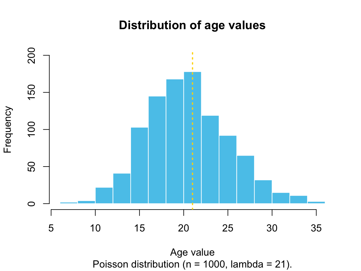
In Chapter 1, we generated a vector age by sampling 1000 random values from a Poisson distribution (see Section 1.6.4):
age <- rpois(n = 1000, lambda = 21)The following plot shows the distribution of age values:68
Suppose we wanted to categorize the age values into three categories “under 18,” “young adult (aged 18 to 30),” and “over 30.”
We could do this by a series of conditionals, but also by using the cut() function with an appropriate setting of its breaks argument:
age_cat <- cut(age, breaks = c(-Inf, 18, 30, +Inf))
levels(age_cat) <- c("under 18", "young adult", "over 30")
(tac <- table(age_cat))
#> age_cat
#>    under 18 young adult     over 30
#>         317         654          29
Note that cut() created a factor variable (assigned to age_cat), whose levels we re-named by assigning levels().
The number of values in each category correspond to cutting the original distribution into three sections (or adding the heights of all bars withing a section into the height of a new bar):
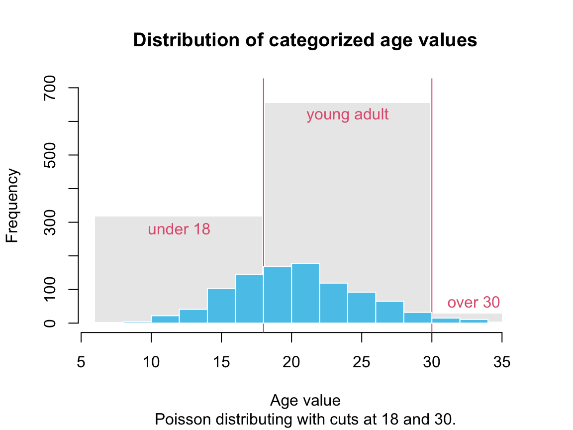
Thus, cut() allows categorizing data into discrete bins.
For more complicated ways of transforming continuous data into categorical data, see the rbin package.
Overall, R provides not only conditional statements, but also various ways of avoiding them. As a consequence, R uses fewer conditionals than most other programming languages. This raises the question: When should we use conditionals? As a general heuristic, we primarily use conditionals in R when the contents of objects are variable and currently unknown (e.g., when writing new functions). By contrast, when working with objects and structures that are fully defined (e.g., rows and columns of existing data), indexing is to be preferred.
Practice
Let’s practice what we have learned about using and avoiding conditionals in R.
1. A conditional nursery rhyme
Consider the following check_flow() function:
check_flow <- function(n) {
  if (is.logical(n)) {return("Logo!")} else
  {print("Ok:")}
  if (length(n) == 1 && is.numeric(n))
  {switch(n,print("ene"),print("mene"),print("miste"),
          print("es rappelt"),print("in der kiste"))
  } else if (is.character(n)) {
    if (is.character(n)) {n <- tolower(n)}
    switch(n,"a" = return("ene"),
           "b" = return("mene"),"c" = return("mu"))
  } else {return("Raus bist du!")}
  "(etc.)"}
The function appears to implement some nursery rhyme, but is really messy, unfortunately.69 Hence, need to clean up this code before we can even begin with trying to understand the function.
- Format the function so that it becomes easier to read and parse.
Solution
A possible solution would indent commands, place any } on a new line, and generally introduce lots of white space, as follows:
check_flow <- function(n) {

  if (is.logical(n)) {
    return("Logo!")
  } else {
    print("Ok:")
  }

  if (length(n) == 1 && is.numeric(n)) {

    switch(n,
           print("ene"),
           print("mene"),
           print("miste"),
           print("es rappelt"),
           print("in der kiste")
    )

  } else if (is.character(n)) {

    if (is.character(n)) {n <- tolower(n)}

    switch(n,
           "a" = return("ene"),
           "b" = return("mene"),
           "c" = return("mu")
    )

  } else {

    return("Raus bist du!")
  }

  "(etc.)"
}
Describe and try to understand the
check_flow()function. What does it do and how does it do it?Answer and predict the results of the following questions:
- Which cases does the 1st conditional statement distinguish?
- When is the 1st
switchstatement reached? When is the 2ndswitchstatement reached?
- What is the difference between the
printand thereturnstatements?
- Under which conditions does the function return
"raus bist du"?
- What happens when you call
check_flow()orcheck_flow(NA)?
- Which cases does the 1st conditional statement distinguish?
- Test your predictions by evaluating the following calls of the
check_flow()function.
Solution
The following expressions are suited to check our check_flow() function:
# Check:
check_flow(2 < 1)
check_flow(2)
check_flow(4)
check_flow(6)
check_flow(8)
check_flow("A")
check_flow("C")
check_flow("ABC")

# Note:
check_flow()  # yields ERROR: argument "n" missing, with no default
check_flow(NA)
check_flow(sqrt(2))
check_flow(pi)
check_flow(4.1)
check_flow(c(1, 2))
check_flow(c("A", "B")) # yields ERROR in switch: EXPR must be a length 1 vector
2. Using switch() without stop()
- What happens with
switch()statements, if the finalstop()argument is omitted and the first argument does not match one of the cases?
Solution
We can easily modify get_i() from above to test this:
get_i <- function(v, i = 1) {

  switch(i,
         v[1],
         v[2],
         v[3],
         warning("Unknown case.")
  )

}

# Check:
get_i(1:10, i = 3)
get_i(1:10, i = 4)  # warning
get_i(1:10, i = 5)  # !!
Using i = 3 and i = 4 yields the expected results.
However, using i = 5 yields no warning (and no error, if we had used stop()).
This illustrates that the final entry of switch() does not work like the else statement in a conditional.
- Try replacing the final
stop()inswitch()withmessage()orwarning(). What changes?
Solution
The following variant of get_i() illustrates the differences:
get_i <- function(v, i = 1) {

  switch(i,
         v[1],
         message("Unknown case 1"),
         warning("Unknown case 2"),
         stop("Unknown case 3")
  )

  print("This line is reached.")

}

# Check:
get_i(1:10, 1)
get_i(1:10, 2)   # message
get_i(1:10, 3)   # warning
get_i(1:10, 4)   # stop (yields error and abandons evaluation)
get_i(1:10, 10)  # !!
This example illustrates the differences between issuing a message(), a warning(), and a stop() (i.e., an error).
Again, the case of i = 10 illustrates that the final entry of switch() does not work like the else statement in a conditional.
3. Recoding variables by ifelse()
In Section 11.3.7, we used logical indexing (rather than conditionals) to recode variables of a data table dt (e.g., for creating a new variable gender). However, perhaps we could have used the vectorized ifelse() function to recode the variable sex as gender?
# Re-create dt:
dt <- tibble::tibble(name, sex, age, height) # re-define dt
dt$gender <- rep(NA, length(dt$sex)) # initialize variable- Would the following expression yield the desired result? Why or why not?
ifelse(dt$sex == "male", dt$gender <- 1, dt$gender <- 2)
dt  # check dt
Solution
The expression fails to work as intended (and all values of dt$sex are set to 2).
Overall, the expression results in the desired vector, but this vector is not assigned to dt$sex.
Instead, all values of dt$gender are set to 2 (which clearly is problematic).
- How could we modify the previous
ifelse()expression to work as intended?
Solution
The following version would work (in this particular case), as a vector of values is assigned to dt$gender:
dt$gender <- ifelse(dt$sex == "male", 1, 2)
dt # check result- Why would logical indexing still be better?
Solution
Using the last ifelse() statement would assign 2 (i.e., “female”) to any record for which dt$sex == "male" is FALSE.
This happens to work in this limited example, but is error-prone in any real environment (which is likely to include additional gender labels).
Thus, using logical indexing is safer, as only cases for which dt$sex == "female" (rather than any non-“male” label) are re-coded as a dt$gender value of 2.
4. More unconditional recoding
Assume we wanted to update two facts in the tibble dt (from above):
a.the height of Eve is measured to be 158cm (i.e., should no longer be NA)
- Adam turned 22 (i.e., his
ageneeds to be adjusted)
- Explain what the following conditionals would do (to a copy
dt2) and why they would fail to make the desired corrections:
dt2 <- dt  # create a copy (to keep original dt)

if (dt2$name == "Eve") {dt2$height <- 158}
if (dt2$name == "Adam")   {dt2$age <-  22}

dt2  # check result
Solution
The tests of both conditionals yield a vector of logical values.
When evaluating them, a warning message informs us that only their first element is used.
As the first element happens to be FALSE for the test dt2$name == "Eve", no height value is being changed.
However, as Adam is the first name on the list, the first element of dt2$name == "Adam" is TRUE and all age values are changed to 22 (due to recycling the dt2$age vector). Overall, the first conditional does not change anything and the second conditional changes too much.
- How could we make the desired corrections?
Solution
A good solution would recode Eve’s height and Adam’s age by logical indexing:
dt2 <- dt  # copy dt

dt2$height[dt2$name == "Eve"] <- 158
dt2$age[dt2$name == "Adam"]   <-  22

dt2  # check result
The following alternatives using ifelse() would also work, but are less elegant than logical indexing:
dt2 <- dt  # copy dt

dt2$height <- ifelse(dt2$name == "Eve", 158, dt2$height)
dt2$age <- ifelse(dt2$name == "Adam", 22, dt2$age)

dt2  # check result
This concludes our practice exercises on conditionals in R. The following section introduces some advanced aspects of R and computer programming (and can be skipped on a first reading of this chapter).
Even using functions implies a linear evaluation on some level. For instance, any function needs to be defined or loaded before it can be used.↩︎
In this case, the values of
agewere created as integer values (from a Poisson distribution), but creating them as continuous values would make no difference for our present purposes.↩︎Actually, this example illustrates pretty well how the functions of students tend to look when they first start writing functions. Imagine searching for a typo in code formatted like this…↩︎