11.4 Advanced aspects of functions
This section introduces four slightly more advanced topics in the context of computer programming:
a programming technique known as recursion (Section 11.4.1),
algorithms for sorting elements (Section 11.4.2),
a way of vectorizing functions (Section 11.4.3), as well as
basic methods for measuring the performance of functions (Section 11.4.4).
These topics are of general interest when learning to program, but we will address them from the perspective of R as our current toolbox for tackling computational tasks. As computers have become incredibly fast and contemporary programming languages provide many functions for solving problems that can be addressed by these techniques, the continued interest in these topics is partly motivated by theoretical considerations. They help us think more carefully about data structures, the flow of control, and the contents of variables when calling functions. Ultimately, considering the process by which functions solve their tasks enables us to create more flexible, efficient, and useful functions.
11.4.1 Recursion
Recursion is the process of defining a problem (or the solution to a problem) in terms of a simpler version of itself. More precisely, recursion solves a problem by (a) identifying a basic solution and (b) recursing more complex cases in small steps towards this solution. As this definition seems circular, people often play on the recursive nature of recursion (e.g., by titles like To understand recursion you have to understand recursion…).
In computer science, recursion is a programming technique involving a function (or algorithm) that calls itself. To avoid getting lost in an infinite loop, the function’s call to itself typically contains a simpler version of the original problem and re-checks a condition that can stop the process when the condition is met. Using this method results in a characteristic process in which successive iterations are executed up to a stopping criterion. Once this criterion is met, all iterations are unwound in the opposite direction (i.e., from the last element called to the first).
Examples
A familiar instance of recursion occurs when you position yourself between two large mirrors and see your image multiplied numerous times. This phenomenon can also be observed when viewing a live recording of yourself in a screen, as illustrated by the xkcd clip shown in Figure 11.2.

Figure 11.2: A recursive explanation of recursion (from xkcd).
An image containing itself as part of the image will inevitably get lost in an infinite regress. In order work as an algorithm, however, a recursive function must include a stopping criterion. Examples of recursive definitions of procedures that include such a condition include:
The task “go home” can be implemented as:
- If you are at home, stop moving.
- Else, move one step towards your home; then go home.
The task “read a book” can be implemented as:
- If you read the last page, stop reading.
- Else, read the current page, then read the rest of the book.
Mathematical definitions: The factorial of a natural number \(n\) is defined as:
- \(n! = n \cdot (n - 1)!\) for \(n > 1\), and
- \(n! = 1\) for \(n = 1\).
- \(n! = n \cdot (n - 1)!\) for \(n > 1\), and
These examples illustrate that a recursive solution typically contains two parts: (1) A stopping case that checks some criterion and stops the process when the criterion is met, and (2) an iterative case that reduces the problem to a simpler version of itself. More specifically, all these examples included three elements: (a) a stopping condition, (b) a simplification step, and (c) a call of the function (instruction, procedure, or task) to itself. However, the three elements were not always presented in the same order. For instance, the mathematical definition of the factorial (above) provided the simplification step (b) and call to itself (c) prior to the stopping condition (a). This sequence may work for mathematical definitions, but can create problems in programming (e.g., when we have to test for a stopping criterion prior to the other steps).
We can easily find additional examples for recursive processes (e.g., solving a complex problem by solving its sub-steps, eating until the plate is empty, etc.). Note that recursion is closely related to many heuristics — strategies that aim to successfully solve a problem in a fast and frugal fashion (i.e., without trying to optimize). For instance, the strategies of divide-and-conquer and hill climbing try to solve a problem by breaking it down into many similar, but simpler ones, and aim to reach the overall goal in smaller steps.
In programming, using recursion is particularly popular when solving problems that involve linear data structures (e.g., vectors or lists, but also strings of text), as these can easily be simplified into smaller sub-problems.
For instance, we can always separate a vector v into its first element v[1] plus its rest v[-1], so that c(v[1], v[-1]) == v:
(v <- letters[1:5])
#> [1] "a" "b" "c" "d" "e"
c(v[1], v[-1])
#> [1] "a" "b" "c" "d" "e"
Essentials of recursion
How recursion works in practice is perhaps best explained by viewing an example. Here is a very primitive recursive function:
recurse <- function(n = 1){

  if (n == 0){return("wow!")}

  else {
    recurse(n = n - 1)
  }
}

# Check:
recurse()
#> [1] "wow!"
recurse(10)
#> [1] "wow!"
The recurse() function is recursive, as it contains a call to itself (in the else part of a conditional statement).
However, note that the inner function call is not identical to the original definition:
It varies by changing its numeric argument from n to n - 1.
Importantly, this small change creates an opportunity for the stopping criterion of the if-statement to become TRUE.
For if n == 0, the then-part of the conditional {return("wow!")} is evaluated.
(If the function called recurse(n = n) from its else-statement, it would call itself an infinite number of times and never stop.)
Our two calls to recurse() and recurse(10) yield the same result, but substantially differ in the way they obtained this result:
By using the function’s default argument of
n = 1, callingrecurse()merely called itself once before meeting the stopping criterion.By contrast,
recurse(10)called itself 10 times beforen == 0became TRUE.
A key insight regarding recursion concerns the question:
- What happens, when the stopping criterion of a recursive function is reached?
A tempting, but false answer would be: The process stops by evaluating the then-part of the conditional (i.e., here: {return("wow!")}).
Although it is correct that this part is evaluated when the stopping criterion is reached, the overall process does not stop there (despite the return() statement).
To understand what actually happens at and after this point, consider the following variation of the recurse() function:
recurse <- function(n = 1){

  if (n == 0){return("wow!")}

  else {
    paste(n, recurse(n = n - 1))
  }
}

# Check:
recurse(0)
#> [1] "wow!"
recurse()
#> [1] "1 wow!"
recurse(10)
#> [1] "10 9 8 7 6 5 4 3 2 1 wow!"
In this more typical variant of a recursive function, we slightly modified the else-part of the conditional.
The results of the evaluations show that the overall process was not finished when the stopping criterion was met and return("wow!") was reached.
As this part is only reached for calling recurse(n = 0), any earlier calls to recurse(n = 1), recurse(n = 2), etc., are still ongoing when return("wow!") is evaluated. Thus, the expression paste("o", recurse(n = n - 1)) is yet to be evaluated n times, which results in adding the current value of n exactly n times to the front of “wow!”
Thus, only the final statement returned by recurse(0) would be “wow!” as — in this particular case of n = 0 — we would never reach the recursive call in the else-part of the conditional.
By contrast, calling recurse(n) for any n > 0 still needs to unwind all recursive loops after reaching the stopping criterion and eventually return the result of the first paste(n, recurse(n - 1)) function.
Actually, there is nothing unusual or mysterious about this. For instance, when writing a nested function like:
paste(3, paste(2, paste(1, "wow!")))
#> [1] "3 2 1 wow!"
we also know and trust that an R compiler parses it by first evaluating its innermost expression paste(1, "wow!"), before evaluating the other (and outer) two paste() functions.
The result ultimately returned by the expression is the result of its outmost function.
Overall, we see that reaching the stopping criterion in a recursive function brings the recursive calls to an end, but the output of calling the recursive function is yet to be determined by the path that led to this point.
The following Figure 11.3 illustrates a recursive process in a graphical fashion.
It is implemented as a recursive plotting function that creates a new plot when n == 0. Thus, the algorithm first prints “Stop!” and “n = 0” in the center, before exiting the recursive calls and printing n rectangles of increasing sizes for values of n > 0:
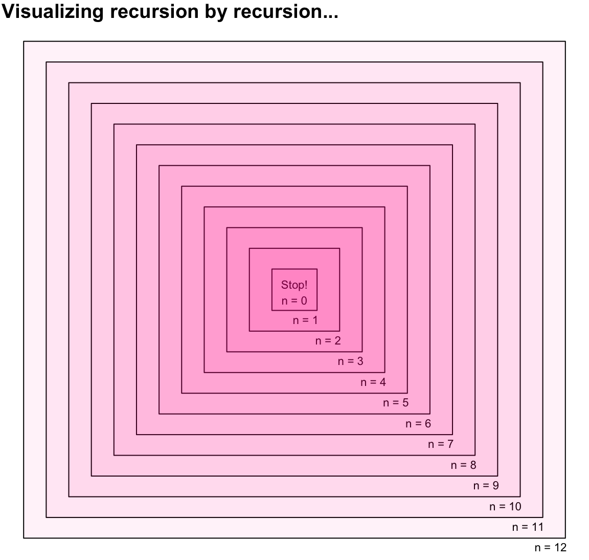
Figure 11.3: Illustrating a recursive process by a recursive plotting function.
Practice
The recurse() function allows to further probe our understanding of recursion:
- Predict the results of the following function calls, then verify your prediction by evaluating them:
recurse(NA)
recurse(-1)- Modify the
recurse()function so that it returns"wow!"with a variable number of final exclamation marks. Specifically, the number of final exclamation marks should indicate the number of recursive function calls to itself. For instance:
recurse()
#> [1] "wow!"
recurse(4)
#> [1] "wow!!!!"
Examples of recursive functions in R
Our recurse() function may have illustrated the principle of recursion, but its uses are rather limited.
To show that recursion can be a useful and powerful programming technique,
here are some examples of problems that can be solved by using recursion in R.
Each example starts out with a task and is then addressed by a recursive solution.
1. Computing the factorial of a natural number n
Task: Define a function fac() that takes a natural number \(n\) as its only argument and computes the result of \(n!\):
fac <- function(n){

  if (n==1) {1}          # stopping condition

  else {n * fac(n - 1)}  # simplify & recurse

}

# Check:
fac(1)
#> [1] 1
fac(5)
#> [1] 120
fac(10) == factorial(10)
#> [1] TRUE
The fac() function implements the above definition of the factorial of a natural number \(n\) in a recursive fashion. For any \(n > 1\), the function computes the product of \(n\) and the factorial of \(n - 1\). The latter factor implies a recursive call to a simplified version of the original problem. These calls iterate to increasingly smaller values of \(n\) until the stopping criterion of \(n=1\) is reached.
Note:
base R provides a
factorial()function that appears to do the same. However,factorial()does not use recursion in its definition, but agamma()function that also works for non-integers.Our recursive definition for
fac()is simple and elegant. But for practical purposes, we may want to verify its input argument before starting the recursive loop. For instance, we could add someifstatements that catch the following cases without breaking ourfac()function:
# Note errors for:
fac(NA)
fac(1/2)
A version of fac() that accommodates these additional cases could look as follows:
Note that fac_rev() still calls fac(), rather than itself.
This is possible here, as the input verification based on the value of \(n\) only needs to occur once.
However, we also could recursively invoke fac_rev() if we wanted to check its inputs whenever the function is called.
2. Reversing a vector
Task: Define a function reverse() that reverses the elements of a vector v:
reverse <- function(v){

  if (length(v) == 1) {v}         # stopping condition

  else {c(reverse(v[-1]), v[1])}  # simplify & recurse

}

# Check:
reverse(c("A", "B", NA, "D"))
#> [1] "D" NA  "B" "A"
reverse(1:5)
#> [1] 5 4 3 2 1
reverse(NA)
#> [1] NA
The crux of the reverse() function lies in its simplification step:
We take the first element v[1], and move it to the end of the reversed rest of the vector v[-1]. As reversing a scalar (i.e., a vector of length 1) leaves v unchanged, this serves as the stopping criterion.
Note:
- base R also contains a
rev()function.
3. Computing the n-th number in the Fibonacci sequence
According to Wikipedia, the series of Fibonacci numbers is characterized by the fact that the \(n\)-th number in the series is the sum of its two preceding numbers (for \(n \geq 2\)). Formally, this requires specifiying the initial numbers and implies:
- Definition: \(F(0)=0\); \(F(1)=1\); \(F(n) = F(n-1) + F(n-2)\) for \(n>1\).
Thus, the first \(20\) values of the Fibonacci sequence are:
- \(0, 1, 1, 2, 3, 5, 8, 13, 21, 34, 55, 89, 144, 233, 377, 610, 987, 1597, 2584, 4181, 6765, ...\)
Task: Define a function fib() that computes the \(n\)-th Fibonacci number.
Here is a recursive definition of a corresponding fib(n) function:
fib <- function(n){

  if (is.na(n)) return(NA)

  if (n==0) {0}       # stop 1

  else if (n==1) {1}  # stop 2

  else {fib(n - 1) + fib(n - 2)}  # 2 recursive calls

}

# Check:
fib(0)
#> [1] 0
fib(1)
#> [1] 1
fib(20)
#> [1] 6765
fib(NA)
#> [1] NA
Note that the definition of our fib() function specifies two stopping criteria (for fib(0) and fib(1)) and its
final else part includes two recursive calls to itself, both of which pose a simpler version of the original problem.
In Chapter 12, we will solve the same problem in an iterative fashion (see Exercise 1, Section 12.5.1). This will show that recursion is closely related to the concept of iteration (i.e., proceeding in a step-wise fashion): Actually, recursion is a special type of iteration, as it employs iteration in an implicit way: By writing functions that call themselves we create loops without defining or labeling them explicitly.
Practice
The following exercises reflect upon the above examples of recursive functions:
- We stated above that a vector
vcan always be separated into its first elementv[1]plus its restv[-1], so thatc(v[1], v[-1]) == v. This may be true for longer vectors, but does it also hold for very short vectors likev <- 1orv <- NA?
Solution
v <- 1
c(v[1], v[-1]) == v
#> [1] TRUE

v <- NA
c(v[1], v[-1]) == v
#> [1] NA

v <- NULL
c(v[1], v[-1]) == v
#> logical(0)
is.null(c(v[1], v[-1]))
#> [1] TRUE
Why do some of the recursive functions defined here (e.g.,
fib()) contain an expressionif (is.na(n)) return(NA), whereas others (e.g.,reverse()) do not have it? Can we reduce this expression toif (is.na(n)) {NA}?Let’s further improve and explore our
fac()function (defined above):Create a revised version
fac_2()that does not cause errors for missing (i.e.,NA) or non-integer inputs (e.g.,n = .5).Our
fac()function included two implicit end points (in theifandelseparts). Define a variantfac_2()that renders all return elements explicit by adding correspondingreturn()statements.
Solution
fac_2 <- function(n){

  # Verify inputs:
  if (is.na(n)) {return(NA)}

  if (n < 0 | !ds4psy::is_wholenumber(n)){
    return(message("fac: n must be a positive integer."))
  }

  # Main:
  if (n==1) {return(1)}     # stopping condition
  return(n * fac_2(n - 1))  # simplification & recursion

}
Checking our function:
fac_2(1)
fac_2(5)
fac_2(NA)
fac_2(1/2)- Write a recursive function
rev_char()that reverses the elements (characters) of a character strings:
Solution
Note that our reverse() function and the base R function rev() work on multi-element objects (i.e., typically vectors), whereas we want to reverse the characters within objects (i.e., change the objects, rather than just their order).
We can still apply the same principles as in our recursive version of reverse(), but need to use paste0() and substr() functions (see Section 9.3) to deconstruct and re-assemble character objects:
rev_char <- function(s){

  if (is.na(s)) {return(NA)}

  if (nchar(s) == 1) {s}

  else {paste0(rev_char(substr(s, 2, nchar(s))), substr(s, 1, 1))}

}
Checking our function:
rev_char("Hello world!")
rev_char("123 NA xyz")
rev_char(NA)
Note that our recursive versions of fib(), fac(), and rev_char() do not work well for vector inputs.
We will address the issue of vectorizing functions below (in Section 11.4.3).
11.4.2 Sorting
The task of sorting elements or objects is one of the most common illustrations for the wide range of computer algorithms and comparisons between different ones.
In R, we may typically want to sort the elements of a vector, or the rows or columns of a table of data.
In the previous chapters, we have seen that R and R packages provide various functions for tackling such tasks (e.g., see the base R functions order() and sort(), or the dplyr functions arrange() and select()).
However, how would we solve such tasks if we were writing our own functions?
The basic task of sorting a set of elements on some dimension can be addressed and solved in many different ways. Different approaches can be used to illustrate the efficiency of different algorithms — and provide us with an opportunity for measuring performance (e.g., by counting steps or timing the execution of tasks).
Essentials on sorting
If we wanted to sort the elements of a vector in R, we could simply use the sort() function provided by base R:
set.seed(101)
(v <- sample(1:100, 5))
#> [1] 73 57 46 95 81

sort(v)
#> [1] 46 57 73 81 95
Alternatively, we could write our own sorting function, if we saw a need to do so.70 But now that we can write our own functions, we should be aware that not all functions are created equal.
For instance, consider the following “solution” to the sorting problem (created in this blog post, for illustrative purposes):
bogosort <- function(x) {

  while(is.unsorted(x)) x <- sample(x)

  x
}

# Check:
bogosort(v)
#  [1] 46 57 73 81 95
If the while() loop confuses us (as we have not yet covered iteration), we can re-write the function using recursion:
bogosort_rec <- function(x) {

  if (!is.unsorted(x)) {x}

  else {bogosort_rec(x = sample(x))}

}

# Check:
bogosort_rec(v)
#  [1] 46 57 73 81 95
Note that the else part in a recursive definition typically calls the same function with a simplified version of the problem. Here, however, the “simplification” consisted merely in replacing the argument x by sample(x).
Thus, we were merely starting over again with a different random permutation of x.
As both bogosort() functions solve our task, it may seem that we have solved our problem.
This is true, as long as we only want to sort the vector v containing 5 elements 73, 57, 46, 95, 81.
However, functions are usually not written for solving just one particular problem — and their performance critically depends on the type and size of problems they are solving.
For the simple problem of sorting v, these erratic versions of a sorting algorithm may have worked. But if our problem had only been slightly more complicated, the same functions may have failed. For instance, if our vector v contains 10 or more elements, the processing times of bogosort(v) become painfully slow, and bogosort_rec(v) even throws error messages that inform us that stack usage is too close to the limit (try this for yourself).
Hence, for creating more flexible functions that can tackle a wider range of problems, efficiency considerations become important.
1. Selection sort algorithm
The basic idea of the so-called selection sort algorithm is to select the smallest element of a set and move it to the front, before sorting the remaining elements. This idea can easily be translated into the two parts of a recursive definition:
Stopping criterion: Sorting
xis trivial whenxonly contains one element.Simplify and recurse: Move the minimum element to the front, and sort the remaining elements.
Implementing these steps in R is simple:
sort_select <- function(x) {

  if (length(x) == 1) {x}

  else {

    ix_min <- which.min(x)

    c(x[ix_min], sort_select(x[-ix_min]))

  }
}
Note that which.min(x) yields the index or position of the first minimum of x (i.e., which(min(v) == v)[1]).
Let’s check our sort_select() function on a vector v:
set.seed(101)
(v <- sample(1:100, 20))
#>  [1] 73 57 46 95 81 58 61 60 59  3 32  9 31 93 53 92 49 14 76 45
# [1] 73 57 46 95 81 58 61 60 59 3 32 9 31 93 53 92 49 14 76 45

(sv <- sort_select(v))
#>  [1]  3  9 14 31 32 45 46 49 53 57 58 59 60 61 73 76 81 92 93 95

# Note:
sort_select(c(1, 2, 2, 1))
#> [1] 1 1 2 2
sort_select(NA)
#> [1] NA
# sort_select(c("A", "C", "B"))  # would yield an error.
As using which.min(x) requires a numeric argument x, our sort_select() function fails for non-numeric inputs (e.g., character vectors).
2. Quick sort algorithm
One of the most famous sorting algorithm is aptly called Quick sort. To understand its basic idea, watch its following enactment (created by Sapientia University, Tirgu Mures (Marosvásárhely), Romania, under the direction of Kátai Zoltán and Tóth László):
As the dance illustrates, the basic idea of the Quick sort algorithm is recursive again:
Stopping criterion: Sorting
xis trivial whenxonly contains one element.Simplify and recurse: Find a pivot value
pvfor the unsorted set of numbersxthat splits it into two similarly sized subsets. Sort all numbers that are smaller than the pivot to the left of the pivot element, and all numbers that are larger than the pivot to the its right. Then call the same function twice — once for each subset.
Implementing these steps in R is simple again:
sort_quick <- function(x) {

  if (length(x) == 1) {x}

  else {

    pv <- (min(x) + max(x)) / 2  # pivot to split x into 2 subsets

    c(sort_quick(x[x < pv]), x[x == pv], sort_quick(x[x > pv]))

  }
}
Let’s check our sort_quick() function on the vector v (from above):
(sv <- sort_quick(v))
#>  [1]  3  9 14 31 32 45 46 49 53 57 58 59 60 61 73 76 81 92 93 95

# Note:
sort_quick(NA)
#> [1] NA
# sort_quick(c(1, 2, 2, 1))  # would yield an error!
# sort_quick(c("A", "C", "B"))  # would yield an error.
Comparing algorithms
We now have created three different algorithms that seem to work fine for the task of sorting numeric vectors. This is not unusual. We can easily see that any particular algorithm can always be tweaked in many different ways. This can be generalized into an inportant insight: There always exists an infinite number of possible algorithms for solving a computational task. Thus, the fact that an algorithm gets a task done may be a necessary condition for being a good algorithm, but it cannot be a sufficient one.
When multiple algorithms get a particular job done, the next question to ask is: How do they differ? To learn more about them, we could vary the range of problems that they need to solve. Provided that all functions are correct, they should always yield the same results. However, seeing how they perform on a large variety of problems may reveal some boundary cases that illustrate how the algorithms differ in some respect. Alternatively, we could solve the same (set of) problem(s) by all algorithms and directly measure some variable that quantifies some aspect of their performance.
11.4.3 Vectorizing functions
As vectors are the main data structure of R, it is considered good practice to accommodate vector inputs when programming in R. However, as we usually tend to think in terms of a specific problem at hand when creating a new function, we often fail to meet this requirement.
For instance, note that our fib() and fac() functions — despite their recursive elegance — would not work seamlessly for vector inputs:
# Using non-vectorized functions with vector inputs:
fib(c(6, 9))
#> [1] 8
fac(c(6, 9))
#> [1]   720 15120
We see that — when providing vector inputs to non-vectorized functions — we may be lucky to obtain the desired results.
However, we sometimes may only receive partial results (here: for fib(c(6, 9))) or get unlucky and not receive any results. Additionally, multiple warning messages indicate that we were only considering atomic inputs when using if() statements to check our input properties.
Ensuring that a new function works on vectorized inputs often requires some additional steps.
Before revising a function, we should first reconsider and explicate our expectations regarding the function (e.g., do we want to reverse the character sequence of each element, or also the sequence of elements?).
Once we have clarified the task and purpose of a function, we can try to replace some parts that only work for atomic inputs by more general expressions (e.g., replacing if() by vectorized ifelse() conditionals, see Section 11.3.4).
A convenient way for turning a non-vectorized function into a vectorized version is provided by the Vectorize() function of base R. For instance, we can easily define a vectorized version of rev_char() as follows:
# Vectorizing functions:
fib_vec <- Vectorize(FUN = fib)
fac_vec <- Vectorize(FUN = fac)

# Checking vectorized versions:
fib_vec(c(6, 9))
#> [1]  8 34
fac_vec(c(6, 9))
#> [1]    720 362880
By specifying additional arguments of Vectorize() we can limit the arguments to be vectorized and adjust some output properties.
More powerful techniques for applying functions to data structures are introduced in Chapter 12 on Iteration (see e.g., Section 12.3 on functional programming).
11.4.4 Measuring performance
So far, our efficiency considerations in the previous sections were mostly abstract and theoretical. By contrast, waiting for some function or program to finish is a very familiar and concrete experience for most programmers and many users, unfortunately.
A more practical approach would require methods for measuring the performance of our functions. Good questions to ask in this context are:
How many times is a function called?
How long does it take to execute it?
R provides multiple ways for answering these questions in a quantitative fashion. In this section, we merely illustrate two basic solutions.
1. Counting function calls
Counting the number of calls to a function (e.g., sort_select()) can be achieved by the trace() function.
Its tracer argument can be equipped with a function that increments a variable count by one:
# Insert a counter into a function:
count <- 0  # initialize

trace(what = sort_select,
      tracer = function() count <<- (count + 1),
      print = FALSE)
#> [1] "sort_select"
Note that the tracer function has no argument, but changes a variable that was defined outside of the function.
This is why the assignment is using the symbol <<-, rather than just <-.
To actually trace our function, we need to use it and then inspect the count variable (after initializing it to 0):
# Test:
count <- 0  # initialize
set.seed(pi)
v <- sample(1:2000, 1000)
head(v)
#> [1]  773 1722  652  999  548  698

sv <- sort_select(v)  # apply function
count                 # check counter
#> [1] 1000

untrace(what = sort_select)  # stops tracing this function
The value of count shows that sort_select() achieved its result by 1000 calls to the function.
Actually, we could have anticipated the result:
Given that sort_select(v) moves the minimum element of v to the front on every function call, it takes length(v) function calls to sort v.
Contrast this with sort_quick():
# Insert a counter into a function:
count <- 0  # re-initialize
trace(what = sort_quick,
      tracer = function() count <<- (count + 1),
      print = FALSE)
#> [1] "sort_quick"

# Test:
sv <- sort_quick(v)  # apply function
count                # check counter
#> [1] 1597

untrace(what = sort_quick)
Thus, sort_quick() requires 1597 calls to sort the 1000 elements of v.
This large value may actually be surprising — at least when knowing that quick sort is considered an efficient algorithm.
However, the fact that the vast majority of calls to sort_quick() result in two calls to the same function lets the counter increase beyond the number of elements in v.
2. Timing function calls
Beyond counting the number of function calls, we may be interested in the time it takes to evaluate an expression. Here is some code for timing the duration of a function call:
options(expressions = 50000)  # Max. number of nested expressions (default = 5000).
# N <- 2000
# set.seed(111)

# v <- runif(N)  # create N random numbers
# head(v)

# Measure run times: ----
system.time(sv <- sort_select(v))
#>    user  system elapsed
#>   0.011   0.003   0.013
system.time(sv <- sort_quick(v))
#>    user  system elapsed
#>   0.005   0.000   0.006
system.time(sv <- sort(v))
#>    user  system elapsed
#>   0.001   0.000   0.000
This shows that — for this particular problem (i.e., the data input v) — sort_quick(v) is considerably faster than sort_select(v). Moreover, despite its additional function calls, the time performance of sort_quick(v)) gets pretty close to the generic base R function sort(), which is typically optimized for our system.
Practice
Here are some practice tasks on sorting algorithms and on evaluating their performance:
Considering ties: Do the above search algorithms also work when the vector
vto be sorted includes ties (i.e., multiple identical elements)? Why or why not?Reconsidering
sort_select(): Write an alternative version ofsort_select()that useswhich.max(), rather thanwhich.min().Reconsidering
sort_quick(): How important is it for the performance ofsort_quick()that the problem is split into two subsets of similar sizes? Find out by writing alternative versions ofsort_quick()that use- (a)
pv <- mean(x) - (b)
pv <- median(x) - (c)
pv <- (min(x) + max(x)) / 3
- (a)
as alternative pivot values. How do these changes affect the performance of the search algorithm?
Hint: As such changes may substantially decrease the performance, we should consider using a simpler test vector v to avoid that our system throws an Error.
Solution
# Define alternative version: ------
sort_quick_alt <- function(x) {

  if (length(x) == 1) {x}

  else {

    pv <- mean(x)    # (a)
    # pv <- median(x)  # (b)
    # pv <- (min(x) + max(x)) / 3  # (c)

    c(sort_quick_alt(x[x < pv]), x[x == pv], sort_quick_alt(x[x > pv]))

  }
}

# Check:
set.seed(1)
v <- sample(1:100, 100)
sort_quick_alt(v)


# Count performance: ------

count <- 0  # initialize

trace(what = sort_quick_alt,
      tracer = function() count <<- (count + 1),
      print = FALSE)

# Test (using v again):
set.seed(101)
sv <- sort_quick_alt(v)  # apply function
count                    # check counter

untrace(what = sort_quick_alt)


# Time performance: ------

system.time(sv <- sort_quick_alt(v))- Vectorizing a function:
Does your
rev_char()function (assigned as an exercise above) also work for vectorized inputs? Verify this by evaluating:
rev_char(c("Hello", "world!"))- If it fails to work or issues multiple warnings, create a vectorized version
rev_char_vec()of it and use this function to verify:
rev_char_vec(c("Hello", "world!"))
#>    Hello   world!
#> "olleH" "!dlrow"- Can you explain and control the names of the vector elements?
This concludes our foray into more advanced aspects of programming in R.
As the functions provided by base R are typically optimized, re-writing such functions rarely makes sense, unless we want to add or change some of its functionality. In this chapter, we are writing alternative
sort()functions for pedagogical reasons.↩︎