12.2 Essentials of iteration
As mentioned in Section 12.1, an iterative task has the general form “for each \(X\), do \(Y\).” Thus, any instruction for an iterative process must specify (a) some data \(X\) and (b) some task(s) \(Y\) that is to be done to each element of \(X\). R provides two general ways for addressing such tasks:
As we focus on the essentials in this book, we will mostly cover basic
forandwhileloops here (see Sections 12.2.1ff.).In more advanced sections, we introduce the notion of functional programming and learn how loops can be replaced by base R’s
apply()(R Core Team, 2021) and purrr’smap()(Henry & Wickham, 2020) family of functions (see Section 12.3).
Taken together, this chapter shows how to use loops for solving repetitive tasks and some alternatives that help explain why more experienced R users often frown upon loops as suboptimal solutions (see Figure 12.3).
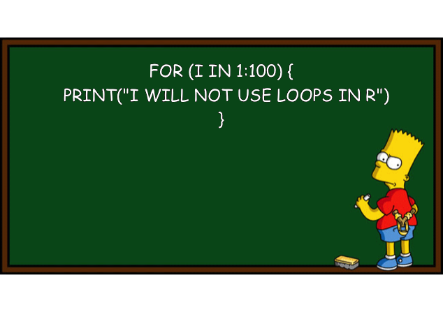
Figure 12.3: Avoiding iteration by a for loop. Do you see the irony in this image? (Image based on this post on the Learning Machines blog and created by the R package meme.)
12.2.1 Basic types of loops
Loops are structures of code that cause some code to be executed repeatedly. In R, we can distinguish between two basic versions:
forloops are indicated when we know the number of required iterations in advance;whileloops are more general and indicated when we only know a condition that should end a loop.
We will discuss both types of loops in the following sections.
#> # A tibble: 6 × 5
#>      id   age height shoesize    IQ
#>   <int> <dbl>  <dbl>    <dbl> <dbl>
#> 1     1    21    173       38    89
#> 2     2    26    193       43    93
#> 3     3    24    171       41    92
#> 4     4    32    191       43    97
#> 5     5    26    156       36   110
#> 6     6    28    172       34   117
12.2.2 Using for loops
When we want to execute some code repeatedly and know the number of required iterations in advance, a for loop is indicated.
Before creating a new loop, we typically need to ask and answer three questions:
Body: What is (or are) the task(s) to be performed (and corresponding code executed) repeatedly?
Sequence: Over which sequence of data elements should be iterated? How many iterations are there?
Output: What is the result of the loop: What type of object and how many instances of them are created?
After answering these questions, a for loop can be designed in reverse order (from output to body):
# (a) prepare output:
output <- vector(<type>, length(start:end))

# (b) for loop:
for (i in start:end) {                    # sequence

  result_i <- <solve task for i-th case>  # body: solve task

  output[[i]] <- result_i                 # collect results in output

}

# (c) use output:
output
Note that the initial output typically is just an empty data structure (e.g., a vector, matrix, or array of NA values) that serves as a placeholder for the results computed within the loop.
Doing something n times
Assuming that we know how often we want to do something (e.g., n times), we can simply instruct R to do it 1:n times.
Task: Compute square number of integers from 1 to 10.
Body: Compute the square value of some number
i.Sequence:
ifrom 1 to 10.Output: A vector of 10 numbers.
Implementation:
# (a) prepare output:
output <- vector("double", length(1:10))

# (b) for loop:
for (i in 1:10) {

  sq <- i^2
  print(paste0("i = ", i, ": sq = ", sq))  # for debugging
  output[[i]] <- sq

}
#> [1] "i = 1: sq = 1"
#> [1] "i = 2: sq = 4"
#> [1] "i = 3: sq = 9"
#> [1] "i = 4: sq = 16"
#> [1] "i = 5: sq = 25"
#> [1] "i = 6: sq = 36"
#> [1] "i = 7: sq = 49"
#> [1] "i = 8: sq = 64"
#> [1] "i = 9: sq = 81"
#> [1] "i = 10: sq = 100"

# (c) use output:
output
#>  [1]   1   4   9  16  25  36  49  64  81 100
Note: In the for loop, we use output[[i]], rather than output[i] to refer to the i-th element of our output vector.
Actually, using single brackets [] would have worked as well, but the double brackets [[]] makes it clear that we want to remove a level of the hierarchy and assign something to every single element of output.
(See Ch. 20.5.2 Subsetting recursive vectors (lists) for more details on this distinction.)
Loops over data
In the context of data science, we often want to iterate over (rows or columns) of data tables. Let’s load some toy data to work with:
## Load data:
tb <- ds4psy::tb  # from ds4psy package
# tb <- readr::read_csv2("../data/tb.csv")  # from local file
# tb <- readr::read_csv2("http://rpository.com/ds4psy/data/tb.csv")  # online

# inspect tb:
dim(tb)  # 100 cases x 5 variables
#> [1] 100   5
head(tb)
#> # A tibble: 6 × 5
#>      id   age height shoesize    IQ
#>   <dbl> <dbl>  <dbl>    <dbl> <dbl>
#> 1     1    21    173       38    89
#> 2     2    26    193       43    93
#> 3     3    24    171       41    92
#> 4     4    32    191       43    97
#> 5     5    26    156       36   110
#> 6     6    28    172       34   117
Suppose we wanted to obtain the means of the variables from age to IQ.
We could call the mean function for each descired variable. Thus, repeating this call for each variable would be:
# (a) Means: ----
mean(tb$age)
#> [1] 26.29
mean(tb$height)
#> [1] 177.78
mean(tb$shoesize)
#> [1] 39.05
mean(tb$IQ)
#> [1] 104.85
However, the statement “for each variable” in the previous sentence shows that we are dealing with an instance of iteration here. When dealing with computers, repetition of identical steps or commands is a signal that there are more efficient ways to accomplish the same task.
How could we use a for loop here? To design this loop, we need to answer our 3 questions from above:
Body: We want to compute the mean of 4 columns (
agetoIQ) intb.Sequence: We want to iterate over columns 2 to 5 (i.e., 4 iterations).
Output: The result or the loop is a vector of type “double,” containing 4 elements.
Notes
We remove the 1st column, as no computation is needed for it.
The i-th column of tibble
tb(or data framedf) can be accessed viatb[[i]](ordf[[i]]).
# Prepare data:
tb_2 <- tb %>% select(-1)
tb_2
#> # A tibble: 100 × 4
#>      age height shoesize    IQ
#>    <dbl>  <dbl>    <dbl> <dbl>
#>  1    21    173       38    89
#>  2    26    193       43    93
#>  3    24    171       41    92
#>  4    32    191       43    97
#>  5    26    156       36   110
#>  6    28    172       34   117
#>  7    20    166       35   107
#>  8    31    172       34   110
#>  9    18    192       32    88
#> 10    22    176       39   111
#> # … with 90 more rows

# (a) prepare output:
output <- vector("double", 4)

# (b) for loop:
for (i in 1:4){

  mn <- mean(tb_2[[i]])

  output[[i]] <- mn

}

# (c) use output:
output
#> [1]  26.29 177.78  39.05 104.85
The range of a for loop can be defined with a special function:
seq_along(tb_2)  # loop through COLUMNS of a df/table
#> [1] 1 2 3 4
The base R function seq_along() returns an integer vector.
When its argument is a table (e.g., a data frame or a tibble), it returns the integer values of all columns, so that the last for loop could be re-written as follows:
# (a) prepare output:
output_2 <- vector("double", 4)

# (b) for loop:
for (i in seq_along(tb_2)){

  mn <- mean(tb_2[[i]])

  output_2[[i]] <- mn

}

# (c) use output:
output_2
#> [1]  26.29 177.78  39.05 104.85
Another way of iterating over all columns of a table tb_2 could loop from 1 to ncol(tb_2):
# (a) prepare output:
output_3 <- vector("double", 4)

# (b) for loop:
for (i in 1:ncol(tb_2)){

  mn <- mean(tb_2[[i]])

  output_3[[i]] <- mn

}

# (c) use output:
output_3
#> [1]  26.29 177.78  39.05 104.85
Practice
- Rewrite the for loop to compute the means of columns 2 to 5 of
tb(i.e., without simplifyingtbtotb_2first).
Solution
We create a new output vector output_4 and need to change two things:
the column numbers of the
forloop statement (from1:4to2:5).the index to which we assign our current mean
mnshould be decreased toi - 1(to assign the mean of column 2 to the 1st element ofoutput_2).
# Using data:
# tb

# (a) prepare output:
output_4 <- vector("double", 4)

# (b) for loop:
for (i in 2:5){

  mn <- mean(tb[[i]])

  output_4[[i - 1]] <- mn

}

# (c) use output:
output_4
#> [1]  26.29 177.78  39.05 104.85

# Verify equality:
all.equal(output, output_4)
#> [1] TRUE- We have learned that creating a
forloop requires knowing (a) the data type of the loop results and (b) a data structure than can collect these results. This is simple and straightforward if eachforloop results in a single number, as then all results can be stored in a vector. However, things get more complicated whenforloops yield tables, lists, or plots, as outputs. Try creating similarforloops that return thesummary()and a histogram (using the base R functionhist()) of each variable intb(or each variable oftb_2).
Solution
Creating a summary():
# (b) Summary: ----
summary(tb$age)
#>    Min. 1st Qu.  Median    Mean 3rd Qu.    Max.
#>   15.00   22.00   24.50   26.29   30.25   46.00
summary(tb$height)
#>    Min. 1st Qu.  Median    Mean 3rd Qu.    Max.
#>   150.0   171.8   177.0   177.8   185.0   206.0
summary(tb$shoesize)
#>    Min. 1st Qu.  Median    Mean 3rd Qu.    Max.
#>   29.00   36.00   39.00   39.05   42.00   47.00
s <- summary(tb$IQ)
s
#>    Min. 1st Qu.  Median    Mean 3rd Qu.    Max.
#>    85.0    97.0   104.0   104.8   113.0   145.0

# What type of object is s?
typeof(s)     # "double"
#> [1] "double"
is.vector(s)  # FALSE
#> [1] FALSE
is.table(s)   # TRUE
#> [1] TRUE
The following for loop is almost identical to the one (computing mean of columns 2:5 of tb) above.
However, we initialize the summaries vector to a mode = "list", which allows storing more complex objects in a vector:
# Loop:
# (a) prepare output:
summaries <- vector(mode = "list", length = 4)  # initialize to a vector of lists!

# (b) for loop:
for (i in 2:5){

  sm <- summary(tb[[i]])

  summaries[[i - 1]] <- sm

}

# (c) use output:
summaries  # print summaries:
#> [[1]]
#>    Min. 1st Qu.  Median    Mean 3rd Qu.    Max.
#>   15.00   22.00   24.50   26.29   30.25   46.00
#>
#> [[2]]
#>    Min. 1st Qu.  Median    Mean 3rd Qu.    Max.
#>   150.0   171.8   177.0   177.8   185.0   206.0
#>
#> [[3]]
#>    Min. 1st Qu.  Median    Mean 3rd Qu.    Max.
#>   29.00   36.00   39.00   39.05   42.00   47.00
#>
#> [[4]]
#>    Min. 1st Qu.  Median    Mean 3rd Qu.    Max.
#>    85.0    97.0   104.0   104.8   113.0   145.0
The following code uses the R command hist() (from the graphics package included in R) to create a histogram for a specific variable (column) of tb:
# Examples of histograms: ----
# hist(tb$age)
# hist(tb$height)
hist(tb_2$shoesize)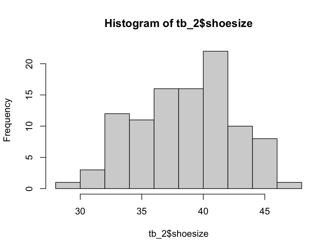
h <- hist(tb$IQ, col = Seeblau) # save graphic as h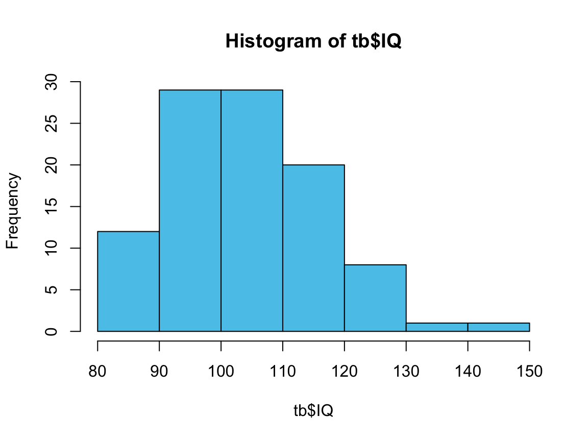
h  # print graphic object
#> $breaks
#> [1]  80  90 100 110 120 130 140 150
#>
#> $counts
#> [1] 12 29 29 20  8  1  1
#>
#> $density
#> [1] 0.012 0.029 0.029 0.020 0.008 0.001 0.001
#>
#> $mids
#> [1]  85  95 105 115 125 135 145
#>
#> $xname
#> [1] "tb$IQ"
#>
#> $equidist
#> [1] TRUE
#>
#> attr(,"class")
#> [1] "histogram"
# plot(h)
The following code uses a loop over the tb_2 data (which was created as tb without the 1st column) to create a histogram for each variable (column) of tb_2. Each histogram is stored in a list out, so that individual plots can be plotted later (using the plot() command on an element of out):
# Data:
tb_2
#> # A tibble: 100 × 4
#>      age height shoesize    IQ
#>    <dbl>  <dbl>    <dbl> <dbl>
#>  1    21    173       38    89
#>  2    26    193       43    93
#>  3    24    171       41    92
#>  4    32    191       43    97
#>  5    26    156       36   110
#>  6    28    172       34   117
#>  7    20    166       35   107
#>  8    31    172       34   110
#>  9    18    192       32    88
#> 10    22    176       39   111
#> # … with 90 more rows
my_blue <- pal_ds4psy[[4]]

# Example:
hist(tb_2[[1]], col = my_blue,
     main = paste0("Histogram of ", names(tb_2[1]), " values:"),
     xlab = names(tb_2[1]))
Four histograms from a for loop:
# For loop:
out <- vector("list", 4)

for (i in seq_along(tb_2)) {  # loop through COLUMNS of tb_2:

  print(i)
  var_name <- names(tb_2[i])
  title <- paste0("Histogram of ", var_name, " values:")
  x_lab <- var_name
  out[[i]] <- hist(tb_2[[i]], col = my_blue,
                   main = title, xlab = x_lab)

}  # end for.
#> [1] 1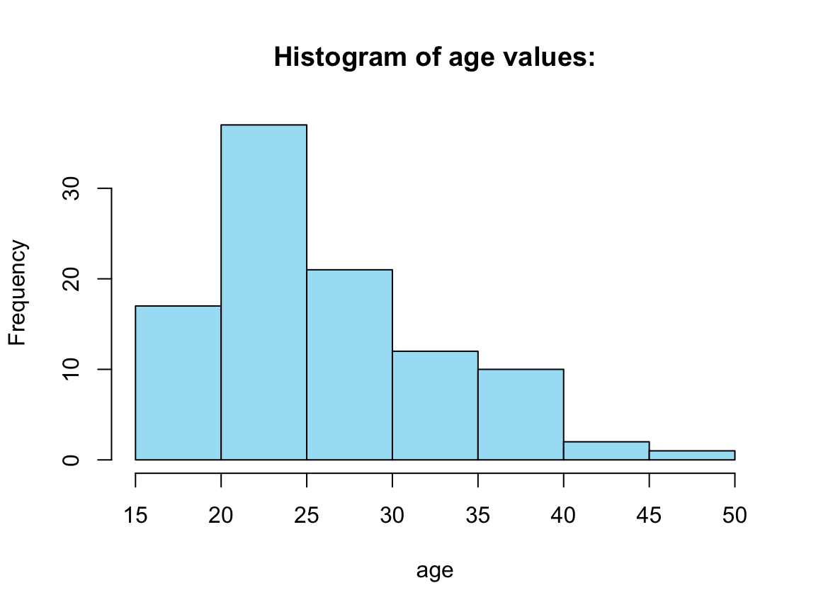
#> [1] 2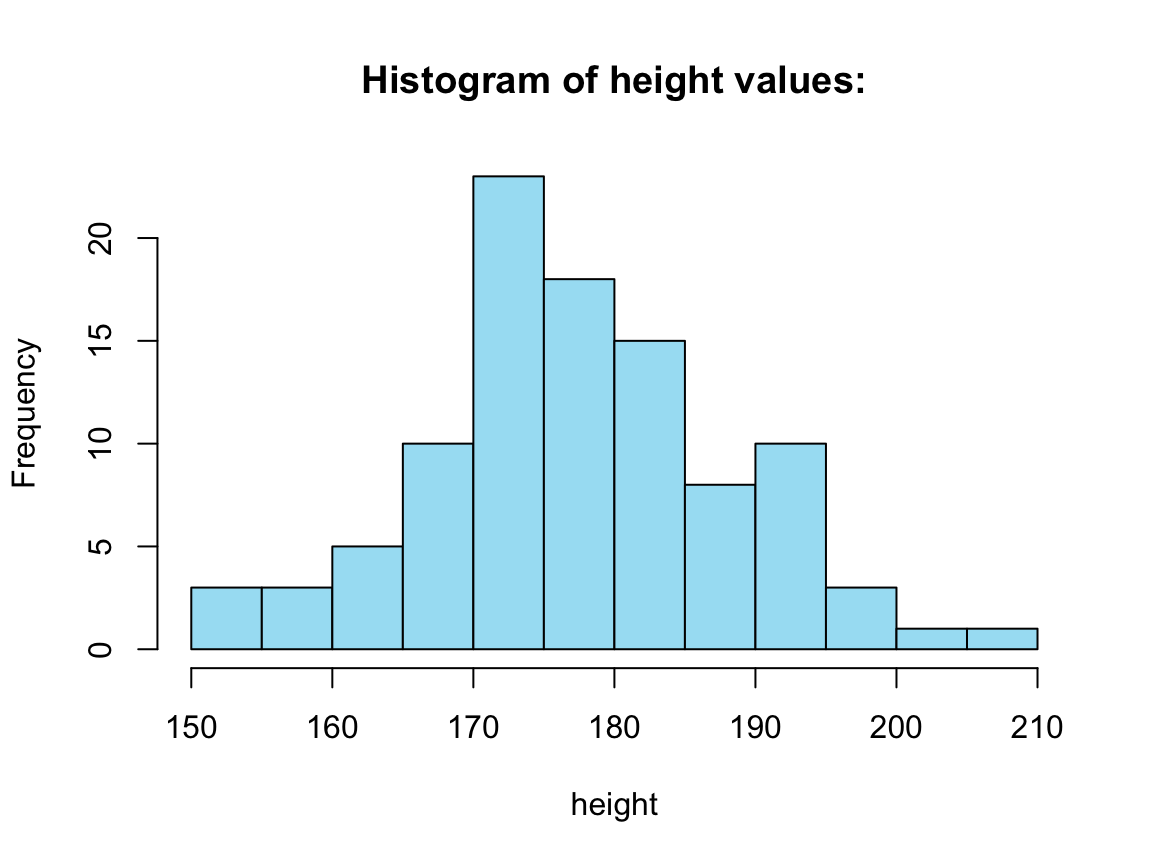
#> [1] 3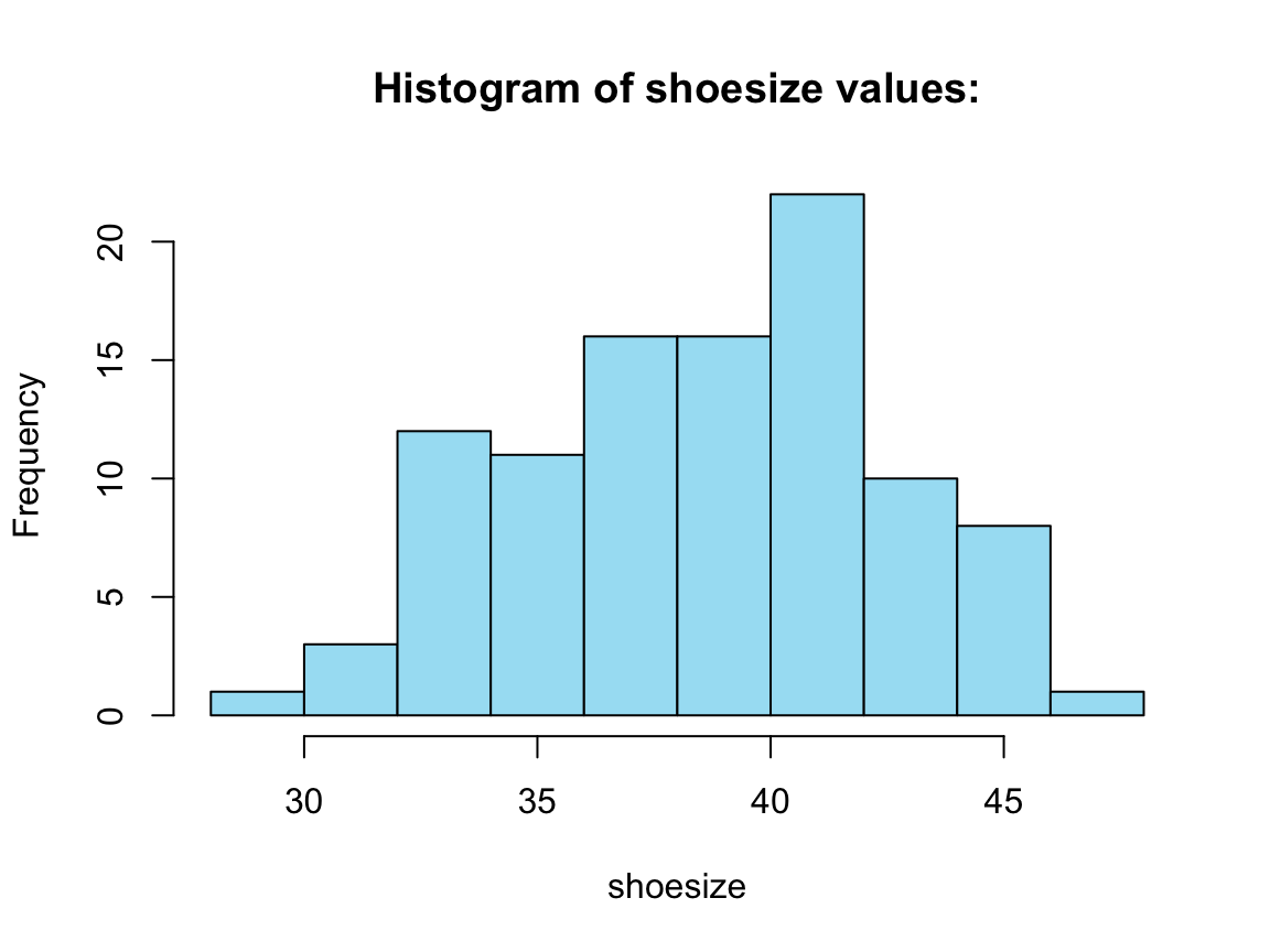
#> [1] 4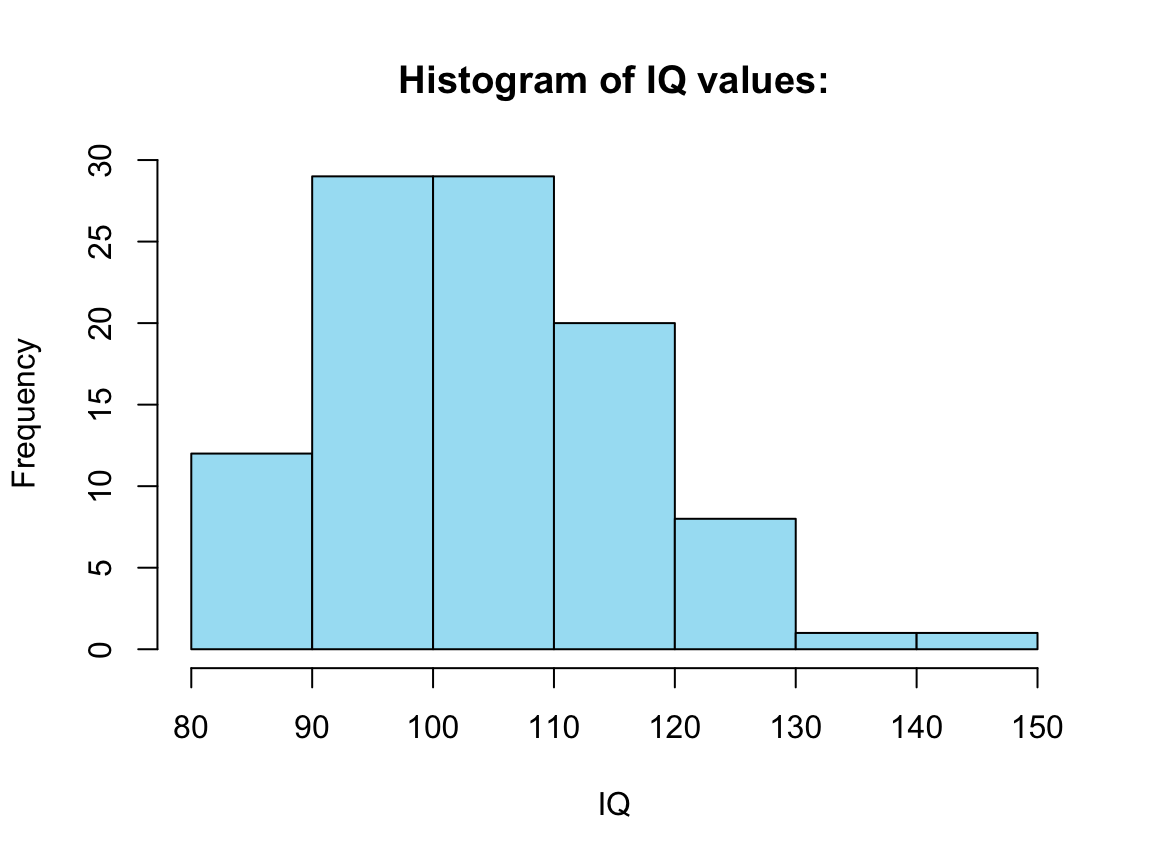
Note that out is a list in which the individual elements are plots.
To view such a plot, we can use the function plot() on elements of the list (remember that we need to use double brackets [[i]] to get the i-th element of a list):
# Plot plots in out:
plot(out[[2]])  # lacks col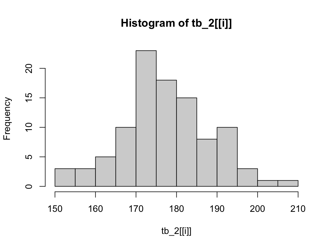
Note that plots in out do lack color, but we can add it (or another one) again:
plot(out[[2]], col = "gold")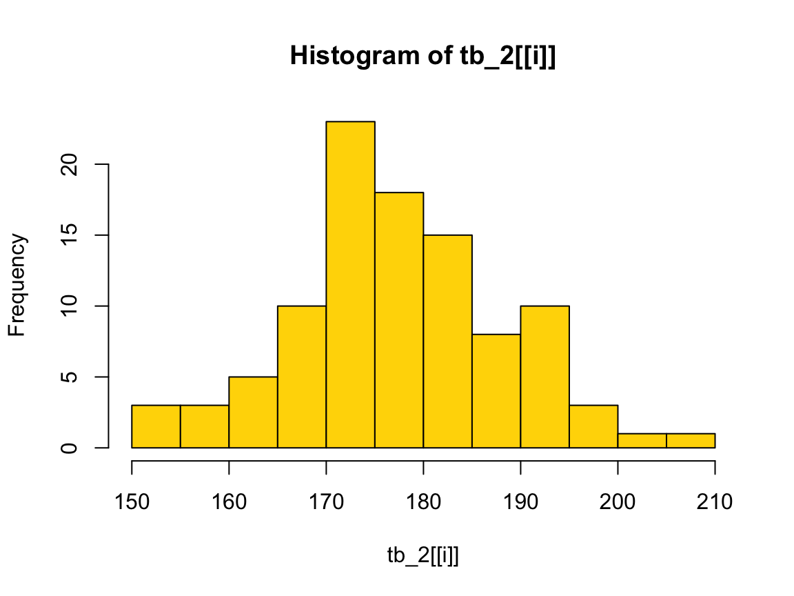
12.2.3 For loop variations
We can distinguish between four variations of the basic theme of the for loop:
1. Modifying an existing object, instead of creating a new object
Example: We want to rescale every column of a table (tibble or data frame).
set.seed(1)  # for reproducible results

tb <- tibble(
  a = rnorm(10),
  b = rnorm(10),
  c = rnorm(10),
  d = rnorm(10)
)
tb
#> # A tibble: 10 × 4
#>         a       b       c       d
#>     <dbl>   <dbl>   <dbl>   <dbl>
#>  1 -0.626  1.51    0.919   1.36
#>  2  0.184  0.390   0.782  -0.103
#>  3 -0.836 -0.621   0.0746  0.388
#>  4  1.60  -2.21   -1.99   -0.0538
#>  5  0.330  1.12    0.620  -1.38
#>  6 -0.820 -0.0449 -0.0561 -0.415
#>  7  0.487 -0.0162 -0.156  -0.394
#>  8  0.738  0.944  -1.47   -0.0593
#>  9  0.576  0.821  -0.478   1.10
#> 10 -0.305  0.594   0.418   0.763

# Define rescale01 function:
rescale01 <- function(x) {
  rng <- range(x, na.rm = TRUE)
  (x - rng[1]) / (rng[2] - rng[1])
}
(a) We could rescale all columns of tb in four separate steps:
df <- tb  # copy

# (a) each column individually:
df$a <- rescale01(df$a)
df$b <- rescale01(df$b)
df$c <- rescale01(df$c)
df$d <- rescale01(df$d)

df
#> # A tibble: 10 × 4
#>          a     b     c     d
#>      <dbl> <dbl> <dbl> <dbl>
#>  1 0.0860  1     1     1
#>  2 0.419   0.699 0.953 0.466
#>  3 0       0.428 0.710 0.645
#>  4 1       0     0     0.484
#>  5 0.479   0.896 0.897 0
#>  6 0.00624 0.582 0.665 0.352
#>  7 0.544   0.590 0.630 0.359
#>  8 0.647   0.848 0.178 0.482
#>  9 0.581   0.815 0.520 0.905
#> 10 0.218   0.754 0.828 0.782
(b) Alternatively, we could use a for loop to modify an existing data structure.
Here are the answers to our three questions regarding loops:
Body: apply
rescale01()to every column oftb.Sequence: A list of columns (i.e., iterate over each column with
seq_along(tb)).Output:
tb(i.e., identical dimensions to the input).
# (b) loop that modifies an existing object:
df2 <- tb  # copy

for (i in seq_along(df2)) {

  df2[[i]] <- rescale01(df2[[i]])

}

# Output:
df2
#> # A tibble: 10 × 4
#>          a     b     c     d
#>      <dbl> <dbl> <dbl> <dbl>
#>  1 0.0860  1     1     1
#>  2 0.419   0.699 0.953 0.466
#>  3 0       0.428 0.710 0.645
#>  4 1       0     0     0.484
#>  5 0.479   0.896 0.897 0
#>  6 0.00624 0.582 0.665 0.352
#>  7 0.544   0.590 0.630 0.359
#>  8 0.647   0.848 0.178 0.482
#>  9 0.581   0.815 0.520 0.905
#> 10 0.218   0.754 0.828 0.782

# Verify equality:
all.equal(df, df2)
#> [1] TRUE
2. Looping over names or values, instead of indices
So far, we used for loop to loop over numeric indices of x with for (i in seq_along(x)),
and then extracted the i-th value of x with x[[i]].
There are 2 additional common loop patterns:
loop over the elements of
xwithfor (x in xs): useful when only caring about side effectsloop over the names of
xwithfor (nm in names(xs)): useful when names are needed for files or plots.
Whenever creating named output, make sure also provide names to the results vector:
x <- 1:3

results <- vector("list", length(x))
names(results) <- names(x)

results
#> [[1]]
#> NULL
#>
#> [[2]]
#> NULL
#>
#> [[3]]
#> NULL
Note that the basic iteration over the numeric indices is the most general form, because given a position we can extract both the current name and the current value:
x <- 1:3

for (i in seq_along(x)) {
  name  <- names(x)[[i]]
  value <- x[[i]]
}
3. Handling outputs of unknown length
Problem: Knowing the number of iterations, but not knowing how long the output will be.
Solution: Increase the size of the output within a loop OR use a list object to collect loop results.
For example, imagine we knew the first N = 1000 digits of pi (i.e., a series of digits 314159 etc.), but wanted to count how frequently a specific target subsequence (e.g., target = 13) occurs in this sequence.
The following code uses pi_100k — available in the ds4psy package or from a file pi_100k.txt —
to read the first N = 1000 digits of pi into a scalar character object pi_1000:
# Data:
## Orig. data source <http://www.geom.uiuc.edu/~huberty/math5337/groupe/digits.html>

pi_100k <- ds4psy::pi_100k  # from ds4psy package

## From local data file:
# pi_all <- readLines("./data/pi_100k.txt")               # from local data file
# pi_data <- "http://rpository.com/ds4psy/data/pi_100k.txt"  # URL of online data file
# pi_100k <- readLines(pi_data)                              # read from online source

N <- 1000
pi_1000 <- paste0(substr(pi_100k, 1, 1), substr(pi_100k, 3, (N + 1)))  # skip the "." at position 2!
nchar(pi_1000)          # 1000 (qed)
#> [1] 1000
substr(pi_1000, 1, 10)  # first 10 digits
#> [1] "3141592653"
The following code uses a for loop to answer the questions: How many times and at which positions does the target <- 13 occur in pi_1000?
# initialize:
count  <-  0  # count number of occurrences
target <- 13
target_positions <- c()  # vector to store positions

# loop:
for (i in 1:(N-1)){

  # Current 2-digit sequence:
  digits_i <- substr(pi_1000, i, i+1)  # as character
  digits_i <- as.integer(digits_i)     # as integer

  if (digits_i == target){

    count <- count + 1  # increment count
    target_positions <- c(target_positions, i)  # add the current i to pi_3

  } # end if.

} # end for.

# Results:
count
#> [1] 12
target_positions
#>  [1] 111 282 364 382 526 599 628 735 745 760 860 972
count == length(target_positions)
#> [1] TRUE
The answers are that 13 occurs 12 times in pi_1000. Its 1st occurrence is at position 111 and its 12-th occurrence at position 972.
Note that we could specify the number of iterations (i.e., N - 1 loops, from 1 to 999), but not the number of elements in target_positions.
Incrementing the target_positions vector by i every time a new target is found — by target_positions <- c(target_positions, i) — is quite slow and inefficient.
However, this is not problematic as long as we only do this once and for a relatively small problem (like a loop with 999 iterations).
A more efficient solutions could initialize target_positions to a list (which can take any data object as an element) and then store any instance of finding the target at the i-th position of pi_1000 as the i-th instance of the list. Once the loop is finished, we can use unlist() to flatten the list to a vector:
# initialize:
count  <- 0   # count number of occurrences
target <- 13
target_positions <- vector("list", (N - 1))  # empty list (of N - 1 elements) to store positions

# loop:
for (i in 1:(N-1)){

  # Current 2-digit sequence:
  digits_i <- substr(pi_1000, i, i+1)  # as character
  digits_i <- as.integer(digits_i)     # as integer

  if (digits_i == target){

    count <- count + 1        # increment count
    target_positions[i] <- i  # add the current i to pi_3

  } # end if.

} # end for.

# Results:
count
#> [1] 12
# target_positions # is a list with mostly NULL
target_positions <- unlist(target_positions)  # flatten list to vector (removing NULL elements)
target_positions
#>  [1] 111 282 364 382 526 599 628 735 745 760 860 972
count == length(target_positions)
#> [1] TRUE
This way, we could initialize the length of target_positions before entering the for loop.
This made it possible to assign any new target to target_positions[i], but made the list much larger than it actually needed to be.
The advantages and disadvantages of these different options should be considered for the specific problem at hand.
4. Handling sequences of unknown length
Problem: The number of iterations is not known in advance.
Solution: Use a
whileloop, with aconditionto stop the loop.
Sometimes we cannot know in advance how many iterations our loop should run for. This is common when dealing with random outcomes or running simulations that need to reach some threshold value to stop.
We can address these problems with a while loop.
Actually, a while loop is simpler than a for loop because it only has two components, a condition and a body:
while (condition) {
  # body
}
A while loop is also more general than a for loop because we can write any for loop as a while loop, but not vice versa.
For instance, any for loop with N steps:
for (i in 1:N){

  # loop body

}
can be re-written as a while loop that uses a counter variable i for the number of iterations and a condition that the maximum number of steps N must not be exceeded:
i <- 1  # initialize counter

while (i <= N){

  # loop body

  i <- i + 1  # increment position counter

}
As this requires explicit maintenance (here: the initialization and incrementation of a counter), we prefer using for loops when the number of iterations is known in advance. However, we often do not know in advance how many iterations we will need
— and that’s what while loops are for.
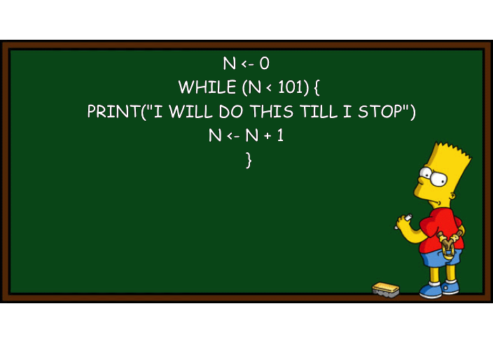
Figure 12.4: Avoiding iteration by using a while loop and a counter. (Image based on this post on the Learning Machines blog and created by the R package meme.)
Example
To illustrate a question, for which we cannot know the number of iterations in advance, we could ask yourselves:
- At which position in the first 1000 digits of pi do we first encounter the subsequence
13?
Actually, we happen to know the answer to this particular problem from computing target_positions above:
The 1st occurrence of 13 in pi_1000 is at position 111.
Knowing a solution makes this an even better practice problem for a while loop.
Assuming that we have no prior information about the sequence to be searched, we cannot solve this sort of problem with a for loop (unless we loop over the entire range of some large sequence, as we did above).
The following while loop solves this task by incrementally increasing an index variable i to inspect the corresponding digits (at positions i and i + 1) of pi_1000 as long as we still want to search (i.e., the condition digits_i != target holds):
# Data:
# pi_1000  # first 1000 digits of pi (from above)

target <- 13
i <- 1  # initialize position counter
digits_i <- as.integer(substr(pi_1000, i, i+1))  # 2-digit integer starting at i

while (digits_i != target){

  i <- i + 1  # increment position counter
  digits_i <- as.integer(substr(pi_1000, i, i+1))  # 2-digit integer starting at i

} # end while.

# Check results:
i  # Position of 1st target:
#> [1] 111
substr(pi_1000, i, i+nchar(target)-1)  # digits at target position(s)
#> [1] "13"
A danger of while loops is that they may never stop. For instance, if we asked:
- At which position in the first 1000 digits of pi do we first encounter the subsequence
999?
we could slightly modify our code above (to accommodate digits_i to look for 3-digit number):
# Data:
# pi_1000  # 1000 digits of pi (from above)

target <- 999    # 3-digit target (found)
# target <- 123  # alternative target (yielding error)

i <- 1  # initialize position counter
digits_i <- as.integer(substr(pi_1000, i, i+2))  # 3-digit integer starting at i

while (digits_i != target){

  i <- i + 1  # increment position counter
  digits_i <- as.integer(substr(pi_1000, i, i+2))  # 3-digit integer starting at i

} # end while.

# Check results:
i  # Position of 1st target:
#> [1] 763
substr(pi_1000, i, i+nchar(target)-1)  # digits at target position(s)
#> [1] "999"
The answer is: The digits 999 first appear at position 763 of pi_1000.
However, if we changed our target to 123 to ask the analog question:
- At which position in the first 1000 digits of pi do we first encounter the subsequence
123?
the same while loop would encounter an error message (try this for yourself):
Error in while (digits_i != target) { :
  missing value where TRUE/FALSE needed
The source of this error becomes obvious when realizing that — when the error is encountered — our index variable`ihas a value of\ 1001: As we simply did not find an instance of\123in the first 1000\ digits of pi, the condition was never met and thewhileloop is now trying to access its 1001.\ digit, which is undefined (NA) forpi_1000and then causes an error in our condition (digits_i != target`).
To prevent this sort of error, we could modify our condition to also stop the while loop after the maximum number of possible steps has been reached. In our case, the while loop only makes sense as long as we do not exceed the number of characters in pi_1000, so that we can add the requirement (i <= nchar(pi_1000)) as an additional (conjunctive, i.e., using &&) test to our condition:
# Data:
# pi_1000  # 1000 digits of pi (from above)

# target <- 999  # 3-digit target (found)
target <- 123    # alternative target (not found)

i <- 1  # initialize position counter
digits_i <- as.integer(substr(pi_1000, i, i+2)) # 3-digit integer starting at position i

while ( (digits_i != target) && (i <= nchar(pi_1000)) ){

  i <- i + 1  # increment position counter
  digits_i <- as.integer(substr(pi_1000, i, i+2)) # 3-digit integer starting at position i

} # end while.

# position of 1st target:
i
#> [1] 1001
This way, the while loop is limited to a maximum of nchar(pi_1000) = 1000 iterations.
If our index variable i shows an impossible value of 1001 after the loop has been evaluated, we can conclude that the target sequence was not found in pi_1000.73
Practice
Knowing or not knowing the number of repetitions for a problem are not always exclusive options. Here is a problem in which both cases appear together:
- Where in
pi_1000are the first three occurrences of the digits13?
Combine a for loop and a while loop to answer this question.
Hint: Inspecting target_positions (computed above) tells you the solution.
But it’s still instructive to combine both type of loops to solve this problem.
# Data:
# pi_1000

# Preparation:
first_3 <- rep(NA, 3)  # initialize output
target <- 13
i <- 1  # initialize position counter
digits_i <- as.integer(substr(pi_1000, i, i+1))  # 2-digit integer starting at i

for (n in seq_along(first_3)){

  while (digits_i != target){

      i <- i + 1  # increment position counter
      digits_i <- as.integer(substr(pi_1000, i, i+1))  # 2-digit integer starting at i

  } # while end.

  first_3[n] <- i  # store current position

  i <- i + 1  # increment position counter
  digits_i <- as.integer(substr(pi_1000, i, i+1))  # 2-digit integer starting at i

} # for end.

# Solution:
first_3

# Verify equality:
all.equal(first_3, target_positions[1:3])
References
Actually, the Error message received before told us as much. However, while such messages are often helpful, programmers should not rely on getting results from errors, as these often have additional effects (e.g., requiring user inputs to further execute a program).↩︎