1.6 Advanced issues
This section introduces some more advanced issues:
Importing data (Section 1.6.1) shows how to read data from files, R packages, or online locations;
Factors (Section 1.6.2) are vectors (variables) that represent categorical data;
Lists (Section 1.6.3) are recursive (hierarchical) vectors that can contain heterogeneous data;
Random sampling (Section 1.6.4) creates vectors by randomly drawing elements from populations or distributions;
Flow control (Section 1.6.5) provides a glimpse on conditional statements and loops in R.
As most of these topics are covered in greater detail in later chapters, this section only serves as a brief introduction or “sneak preview.” So do not panic if some of these topics remain a bit puzzling at this point. Essentially, our current goal is only to become familiar with these concepts and distinctions. It is good to be aware of their existence and recognize them later, even if some details remain a bit fuzzy at this stage.
1.6.1 Importing data
In most cases, we do not generate the data that we analyze, but obtain a table of dataset from somewhere else. Typical locations of data include:
- data included in R packages,
- data stored on a local or remote hard drive,
- data stored on online servers.
R and RStudio provide many ways of reading in data from various sources. Which way is suited to a particular dataset depends mostly on the location of the file and the format in which the data is stored. Chapter 6 on Importing data will examine different ways of importing datasets in greater detail. Here, we merely illustrate the two most common ways of importing a dataset: From a file or from an R package.
The data we import stems from an article in the Journal of Clinical Psychology (Woodworth, O’Brien-Malone, Diamond, & Schüz, 2017). An influential paper by Seligman et al. (Seligman, Steen, Park, & Peterson, 2005) found that several positive psychology interventions reliably increased happiness and decreased depressive symptoms in a placebo-controlled internet study. Woodworth, O’Brien-Malone, Diamond, & Schüz (2017) re-examined this claim by measuring the long-term effectiveness of different web-based positive psychology interventions and published their data in another article (Woodworth, O’Brien-Malone, Diamond, & Schüz, 2018) (see Appendix B.1 for details).
Data from a file
When loading data that is stored as a file, there are 2 questions to answer:
- Location: Where is the file stored?
- Format: In which format is the file stored?
To illustrate how data can be imported from an online source, we store a copy of the participant data from Woodworth, O’Brien-Malone, Diamond, & Schüz (2018) as a text file in CSV (comma-separated-value) format on a web server at http://rpository.com/ds4psy/data/posPsy_participants.csv.
Given this setup, we can load the dataset into an R object p_info by evaluating the following command (from the package readr, which is part of the tidyverse):
p_info <- readr::read_csv(file = "http://rpository.com/ds4psy/data/posPsy_participants.csv")Note the feedback message provided by the read_csv() function of the readr package: It tells us the names of the variables (columns) that were read and the data type of these variables (here: numeric variables of type “double”). To obtain basic information about the newly created tibble p_info, we can simply evaluate its name:
p_info
#> # A tibble: 295 × 6
#>       id intervention   sex   age  educ income
#>    <dbl>        <dbl> <dbl> <dbl> <dbl>  <dbl>
#>  1     1            4     2    35     5      3
#>  2     2            1     1    59     1      1
#>  3     3            4     1    51     4      3
#>  4     4            3     1    50     5      2
#>  5     5            2     2    58     5      2
#>  6     6            1     1    31     5      1
#>  7     7            3     1    44     5      2
#>  8     8            2     1    57     4      2
#>  9     9            1     1    36     4      3
#> 10    10            2     1    45     4      3
#> # … with 285 more rows
Data from an R package
An even simpler way of obtaining a data file is available when datasets are stored in and provided by R packages (aka. libraries).
In this case, some R developer has typically saved the data in a compressed format (as an .rda file) and it can be accessed by installing and loading the corresponding R package. Provided that we have installed and loaded this package, we can easily access the corresponding dataset.
In our case, we need to load the ds4psy package, which contains the participant data as an R object posPsy_p_info.
We can treat and manipulate such data objects just like any other R object. For instance, we can copy the dataset posPsy_p_info into another R object by assigning it to p_info_2:
# install.packages("ds4psy")  # installs the 'ds4psy' package
library(ds4psy)               # loads the 'ds4psy' package

p_info_2 <- posPsy_p_info
Having loaded the same data in two different ways, we should verify that we obtained the same result both times.
We can verify that p_info and p_info_2 are equal by using the all.equal() function:
all.equal(p_info, p_info_2)
#> [1] "Attributes: < Names: 2 string mismatches >"
#> [2] "Attributes: < Length mismatch: comparison on first 3 components >"
#> [3] "Attributes: < Component 2: target is externalptr, current is numeric >"
#> [4] "Attributes: < Component 3: Modes: numeric, list >"
#> [5] "Attributes: < Component 3: Lengths: 295, 3 >"
#> [6] "Attributes: < Component 3: names for current but not for target >"
#> [7] "Attributes: < Component 3: Attributes: < target is NULL, current is list > >"
#> [8] "Attributes: < Component 3: target is numeric, current is col_spec >"
Throughout this book, we will primarily rely on the datasets provided by the ds4psy package or the example datesets included in various tidyverse packages. Loading files from different locations and commands for writing files in various formats will be discussed in detail in Chapter 6 on Importing data.
Checking a dataset
To get an initial idea about the contents of a dataset (often called a data frame, table, or tibble), we typically inspect its dimensions, print it, ask for its structure (by using the base R function str()), or take a glimpse() on its variables and values:
dim(p_info)              # 295 rows, 6 columns
#> [1] 295   6
p_info                   # prints a summary of the table/tibble
#> # A tibble: 295 × 6
#>       id intervention   sex   age  educ income
#>    <dbl>        <dbl> <dbl> <dbl> <dbl>  <dbl>
#>  1     1            4     2    35     5      3
#>  2     2            1     1    59     1      1
#>  3     3            4     1    51     4      3
#>  4     4            3     1    50     5      2
#>  5     5            2     2    58     5      2
#>  6     6            1     1    31     5      1
#>  7     7            3     1    44     5      2
#>  8     8            2     1    57     4      2
#>  9     9            1     1    36     4      3
#> 10    10            2     1    45     4      3
#> # … with 285 more rows
str(p_info)              # shows the structure of an R object
#> spec_tbl_df [295 × 6] (S3: spec_tbl_df/tbl_df/tbl/data.frame)
#>  $ id          : num [1:295] 1 2 3 4 5 6 7 8 9 10 ...
#>  $ intervention: num [1:295] 4 1 4 3 2 1 3 2 1 2 ...
#>  $ sex         : num [1:295] 2 1 1 1 2 1 1 1 1 1 ...
#>  $ age         : num [1:295] 35 59 51 50 58 31 44 57 36 45 ...
#>  $ educ        : num [1:295] 5 1 4 5 5 5 5 4 4 4 ...
#>  $ income      : num [1:295] 3 1 3 2 2 1 2 2 3 3 ...
#>  - attr(*, "spec")=
#>   .. cols(
#>   ..   id = col_double(),
#>   ..   intervention = col_double(),
#>   ..   sex = col_double(),
#>   ..   age = col_double(),
#>   ..   educ = col_double(),
#>   ..   income = col_double()
#>   .. )
#>  - attr(*, "problems")=<externalptr>
tibble::glimpse(p_info)  # shows the types and initial values of all variables (columns)
#> Rows: 295
#> Columns: 6
#> $ id           <dbl> 1, 2, 3, 4, 5, 6, 7, 8, 9, 10, 11, 12, 13, 14, 15, 16, 17…
#> $ intervention <dbl> 4, 1, 4, 3, 2, 1, 3, 2, 1, 2, 2, 2, 4, 4, 4, 4, 3, 2, 1, …
#> $ sex          <dbl> 2, 1, 1, 1, 2, 1, 1, 1, 1, 1, 1, 1, 1, 1, 2, 1, 1, 1, 1, …
#> $ age          <dbl> 35, 59, 51, 50, 58, 31, 44, 57, 36, 45, 56, 46, 34, 41, 2…
#> $ educ         <dbl> 5, 1, 4, 5, 5, 5, 5, 4, 4, 4, 5, 4, 5, 1, 2, 1, 4, 5, 3, …
#> $ income       <dbl> 3, 1, 3, 2, 2, 1, 2, 2, 3, 3, 1, 3, 3, 2, 2, 1, 2, 2, 1, …
Understanding a dataset
When loading a new data file, it is crucial to always obtain a description of the variables and values contained in the file (often called a Codebook).
For the dataset loaded into p_info, this description looks as follows:
posPsy_participants.csv contains demographic information of 295 participants:
id: participant IDintervention: 3 positive psychology interventions, plus 1 control condition:- 1 = “Using signature strengths,”
- 2 = “Three good things,”
- 3 = “Gratitude visit,”
- 4 = “Recording early memories” (control condition).
sex:- 1 = female,
- 2 = male.
age: participant’s age (in years).educ: level of education:- 1 = Less than Year 12,
- 2 = Year 12,
- 3 = Vocational training,
- 4 = Bachelor’s degree,
- 5 = Postgraduate degree.
income:- 1 = below average,
- 2 = average,
- 3 = above average.
Beyond conveniently loading datasets, another advantage of using data provided by R packages is that the details of a dataset are easily accessible by using the standard R help system. For instance, provided that the ds4psy package is installed and loaded, we can obtain the codebook and background information of the posPsy_p_info data by evaluating ?posPsy_p_info.
?posPsy_p_infoOf course, being aware of the source, structure, and variables of a dataset are only the first steps of data analysis. Ultimately, understanding a dataset is the motivation and purpose of its analysis. The next steps on this path involve phases of data screening, cleaning, and transformation (e.g., checking for missing or extreme cases, viewing variable distributions, and obtaining summaries or visualizations of key variables). This process and mindset are described in the chapter on Exploring data (Chapter 4).
Practice
Using the data in
p_info, create a new variableuni_degreethat isTRUEif and only if a person has a Bachelor’s or Postgraduate degree.Use R functions to obtain (the row data of) the youngest person with a university degree.
We will examine this data file further in Exercise 8 (see Section 1.8.8).
1.6.2 Factors
Whenever creating a new vector or a table with several variables (i.e., a data frame or tibble), we need to ask ourselves whether the variable(s) containing character strings or numeric values are to be considered as factors. A factor is a categorical variable (i.e., a vector or column in a data frame) that is measured on a nominal scale (i.e., distinguishes between different levels, but attaches no meaning to their order or distance). Factors may sort their levels in some order, but this order merely serves illustrative purposes (e.g., arranging the entries in a table or graph). Typical examples for factor variables are gender (e.g., “male,” “female,” “other”) or eye color (“blue,” “brown,” “green,” etc.). A good test for a categorical (or nominal) variable is that its levels can be re-arranged (without changing the meaning of the measurement) and averaging makes no sense (as the distances between levels are undefined).
stringsAsFactors = FALSE
Let’s revisit our example of creating a data frame df from the four vectors name, gender, age, and height (see Section 1.5.2).
The columns of this table were originally provided as vectors of type “character.” In many cases, character variables simply contain text data that we do not want to treat as factors. When we want to prevent R from converting character variables into factors when creating a new data frame, we can explicitly set an option stringsAsFactors = FALSE in the data.frame() command:
df <- data.frame(name, gender, age, height,
                 stringsAsFactors = FALSE)  # the new default (as of R 4.0.0)
df
#>     name gender age height
#> 1   Adam   male  21    165
#> 2 Bertha female  23    170
#> 3 Cecily female  22    168
#> 4   Dora female  19    172
#> 5    Eve female  21    158
#> 6   Nero   male  18    185
#> 7   Zeno   male  24    182
Let’s inspect the resulting gender variable of df:
df$gender
#> [1] "male"   "female" "female" "female" "female" "male"   "male"
is.character(df$gender)  # a character variable
#> [1] TRUE
is.factor(df$gender)     # not a factor, qed.
#> [1] FALSE
all.equal(df$gender, gender)
#> [1] TRUE
This shows that the variable df$gender is a vector of type “character,” rather than a factor.
In fact, df$gender is equal to gender, as the original vector also was of type “character.”
stringsAsFactors = TRUE
Up to R version 4.0.0 (released on 2020-04-24), the default setting of the data.frame() function was stringsAsFactors = TRUE. Thus, when creating the data frame df above, the variables consisting of character strings (here: name and gender) were — to the horror of generations of students — automatically converted into factors.26
We can still re-create the previous default behavior by setting stringsAsFactors = TRUE:
df <- data.frame(name, gender, age, height,
                 stringsAsFactors = TRUE)

df$gender  # Levels are not quoted and ordered alphabetically
#> [1] male   female female female female male   male
#> Levels: female male
is.factor(df$gender)
#> [1] TRUE
typeof(df$gender)
#> [1] "integer"
unclass(df$gender)
#> [1] 2 1 1 1 1 2 2
#> attr(,"levels")
#> [1] "female" "male"
In this data frame df, all character variables were converted into factors. When inspecting a factor variable, its levels are printed by their text labels. But when looking closely at the output of df$gender, we see that the labels male and female are not quoted (as the text elements in a character variable would be) and the factor levels are printed below the vector.
Factors are similar to character variables insofar as they identify cases by a text label.
However, the different factor values are internally saved as integer values that are mapped to the different values of the character variable in a particular order (here: alphabetically). The unclass() command shows that the variable names of df are internally saved as integers from 1 to 7 (with the original names as labels of the seven factor levels). Similarly, the gender variable of df contains only integer values of 1 and 2, with 1 corresponding to “female” and 2 corresponding to “male.”
Importantly, a factor value denotes solely the identity of a particular factor level, rather than its magnitude. For instance, elements with an internal value of 2 (here: “male”) are different from those with a value of 1 (here: “female”), but not larger or twice as large.
To examine the differences between factors and character variables, we can use the as.character() and as.factor() functions to switch factors into characters and vice versa.
as.character() turns factors into character variables
Using the as.character() function on a factor and assigning the result to the same variable turns a factor into a character variable:
# (1) gender as a character variable:
df$gender <- as.character(df$gender)
df$gender
#> [1] "male"   "female" "female" "female" "female" "male"   "male"

is.factor(df$gender)    # not a factor
#> [1] FALSE
levels(df$gender)       # no levels
#> NULL
typeof(df$gender)       # a character variable
#> [1] "character"
unclass(df$gender)
#> [1] "male"   "female" "female" "female" "female" "male"   "male"
# as.integer(df$gender) # would yield an error, as undefined for character variables.
We see that using the as.character() function on the factor df$gender created a character variable.
Each element of the character variable is printed in quotation marks (i.e., "female" vs. "male").
as.factor() turns character variables into factors
When now using the function as.factor() on a character variable, we turn the character string variable into a factor.
Internally, this changes the variable in several ways:
Each distinct character value is turned into a particular factor level, the levels are sorted (here: alphabetically), and the levels are mapped to an underlying numeric representation (here: consecutive integer values, starting at 1):
# (2) gender as a factor variable:
df$gender <- as.factor(df$gender)  # convert from "character" into a "factor"
df$gender
#> [1] male   female female female female male   male
#> Levels: female male

is.factor(df$gender)   # a factor
#> [1] TRUE
levels(df$gender)      # 2 levels
#> [1] "female" "male"
typeof(df$gender)      # an integer variable
#> [1] "integer"
as.integer(df$gender)  # convert factor into numeric variable
#> [1] 2 1 1 1 1 2 2
Thus, using as.factor() on a character variable created a factor that is internally represented as integer values. When printing the variable, its levels are identified by the factor labels, but not printed in quotation marks (i.e., female vs. male).
factor() defines factor variables with levels
Suppose we knew not only the current age, but also the exact date of birth (DOB) of the people in df:
| name | gender | age | height | DOB |
|---|---|---|---|---|
| Adam | male | 21 | 165 | 2000-07-23 |
| Bertha | female | 23 | 170 | 1998-12-13 |
| Cecily | female | 22 | 168 | 1999-09-03 |
| Dora | female | 19 | 172 | 2003-03-01 |
| Eve | female | 21 | 158 | 2000-04-19 |
| Nero | male | 18 | 185 | 2003-05-27 |
| Zeno | male | 24 | 182 | 1997-05-16 |
The new variable df$DOB (i.e., a column of df) is of type “Date,” which is another type of data that we will encounter in detail in Chapter 10 on Dates and times.
A nice feature of date and time variables is that they can be used to extract date- and time-related elements, like the names of months and weekdays.
For the DOB values of df, the corresponding variables month and wday are as follows:
| name | gender | age | height | DOB | month | wday |
|---|---|---|---|---|---|---|
| Adam | male | 21 | 165 | 2000-07-23 | Jul | Sun |
| Bertha | female | 23 | 170 | 1998-12-13 | Dec | Sun |
| Cecily | female | 22 | 168 | 1999-09-03 | Sep | Fri |
| Dora | female | 19 | 172 | 2003-03-01 | Mar | Sat |
| Eve | female | 21 | 158 | 2000-04-19 | Apr | Wed |
| Nero | male | 18 | 185 | 2003-05-27 | May | Tue |
| Zeno | male | 24 | 182 | 1997-05-16 | May | Fri |
The two new variables df$month and df$wday presently are character vectors:
df$month
#> [1] "Jul" "Dec" "Sep" "Mar" "Apr" "May" "May"
is.character(df$month)
#> [1] TRUE

df$wday
#> [1] "Sun" "Sun" "Fri" "Sat" "Wed" "Tue" "Fri"
is.character(df$wday)
#> [1] TRUE
If we ever wanted to categorize people by the month or weekday on which they were born or create a visualization that used the names of months or weekdays as an axis, it would make more sense to define these variables as factors.
However, simply using as.factor() on the columns of df would fall short:
as.factor(df$month)
#> [1] Jul Dec Sep Mar Apr May May
#> Levels: Apr Dec Jul Mar May Sep
as.factor(df$wday)
#> [1] Sun Sun Fri Sat Wed Tue Fri
#> Levels: Fri Sat Sun Tue Wed
The resulting vectors would be factors, but their levels are incomplete (as not all months and weekdays were present in the data) and would be sorted in alphabetical order (e.g., the month of “Apr” would precede “Feb”).
The factor() function allows defining a factor variable from scratch.
As must factors can assume a fixed number of levels, the function contains an argument levels to provide the possible factor levels (as a character vector):
# Define all possible factor levels (as character vectors):
all_months <-  c("Jan", "Feb", "Mar", "Apr", "May", "Jun",
                 "Jul", "Aug", "Sep", "Oct", "Nov", "Dec")
all_wdays  <- c("Mon", "Tue", "Wed", "Thu", "Fri", "Sat", "Sun")

# Define factors (with levels):
factor(df$month, levels = all_months)
#> [1] Jul Dec Sep Mar Apr May May
#> Levels: Jan Feb Mar Apr May Jun Jul Aug Sep Oct Nov Dec
factor(df$wday, levels = all_wdays)
#> [1] Sun Sun Fri Sat Wed Tue Fri
#> Levels: Mon Tue Wed Thu Fri Sat Sun
As we explicitly defined all_months and all_wdays (as character vectors) and specified them as the levels of the factor() function, the resulting vectors are factors that know about values that did not occur in the data.
At this point, the factor levels are listed in a specific order, but are only considered to be different from each other. If we explicitly wanted to express that the levels are ordered, we can set the argument ordered to TRUE:
factor(df$month, levels = all_months, ordered = TRUE)
#> [1] Jul Dec Sep Mar Apr May May
#> 12 Levels: Jan < Feb < Mar < Apr < May < Jun < Jul < Aug < Sep < ... < Dec
factor(df$wday,  levels = all_wdays,  ordered = TRUE)
#> [1] Sun Sun Fri Sat Wed Tue Fri
#> Levels: Mon < Tue < Wed < Thu < Fri < Sat < Sun
Thus, if we wanted to convert the variables month and wday of df into ordered factors, we would need to re-assign them as follows:
df$month <- factor(df$month, levels = all_months, ordered = TRUE)
df$wday  <- factor(df$wday,  levels = all_wdays,  ordered = TRUE)
Appearance vs. representation
We just encoded the character variables month and wday of a data frame df as ordered factors.
However, the resulting data frame df looks and prints as it did before:
| name | gender | age | height | DOB | month | wday |
|---|---|---|---|---|---|---|
| Adam | male | 21 | 165 | 2000-07-23 | Jul | Sun |
| Bertha | female | 23 | 170 | 1998-12-13 | Dec | Sun |
| Cecily | female | 22 | 168 | 1999-09-03 | Sep | Fri |
| Dora | female | 19 | 172 | 2003-03-01 | Mar | Sat |
| Eve | female | 21 | 158 | 2000-04-19 | Apr | Wed |
| Nero | male | 18 | 185 | 2003-05-27 | May | Tue |
| Zeno | male | 24 | 182 | 1997-05-16 | May | Fri |
Thus, defining the character variables month and wday of df as ordered factors affects how these variables are represented and treated by R functions, but not necessarily how they appear. The difference between the properties of an underlying representation and its (often indiscriminate and possibly deceptive) appearance on the surface is an important aspect of representations that will pop up repeatedly throughout this book and course.
Note that turning variables into factors affects what we can do with them.
For instance, if month or wday were numeric variables, we could use them for arithmetic comparisons and indexing, like:
df$month > 6        # Who's birthday is in 2nd half of year?
#> [1] NA NA NA NA NA NA NA
name[df$wday == 7]  # Who is born on a Sunday?
#> character(0)
As these variables are factors, however, these statements yield NA values.
as.numeric() turns factor levels into numbers, but…
We could fix this by using the as.numeric() function for converting factor levels into numbers:
# Using factors as numeric variables:
as.numeric(df$month) > 6        # Who's birthday is in 2nd half of year?
#> [1]  TRUE  TRUE  TRUE FALSE FALSE FALSE FALSE
name[as.numeric(df$wday) == 7]  # Who is born on a Sunday?
#> [1] "Adam"   "Bertha"
This seems to work, but requires that we are aware how the factor levels were defined (e.g., that the 7th level of wday corresponded to Sunday). As it is easy to make mistakes when interpreting factors as numbers, we should always check and double check the result of such conversions. Actually, converting factor levels into numbers is often a sign that a variable should not have been encoded as a factor.
The subtle, but profound lesson here is that variables that may appear the same (e.g., when printing a variable or inspecting a data table) may still differ in important ways. Crucially, the type and status of a variable affects what can be done with it and how it is treated by R commands. For instance, asking for summary() on a factor yields a case count for each factor level (including levels without any cases):
# Summary of factors:
summary(df$month)
#> Jan Feb Mar Apr May Jun Jul Aug Sep Oct Nov Dec
#>   0   0   1   1   2   0   1   0   1   0   0   1
summary(df$wday)
#> Mon Tue Wed Thu Fri Sat Sun
#>   0   1   1   0   2   1   2
By contrast, calling summary() on the corresponding numeric variables yields descriptive statistics of its numbers:
# Summary of numeric variables:
summary(as.numeric(df$month))
#>    Min. 1st Qu.  Median    Mean 3rd Qu.    Max.
#>   3.000   4.500   5.000   6.429   8.000  12.000
summary(as.numeric(df$wday))
#>    Min. 1st Qu.  Median    Mean 3rd Qu.    Max.
#>     2.0     4.0     5.0     5.0     6.5     7.0
and a summary() of the corresponding character variables merely describes the vector of text labels:
# Summary of character variables:
summary(as.character(df$month))
#>    Length     Class      Mode
#>         7 character character
summary(as.character(df$wday))
#>    Length     Class      Mode
#>         7 character character
Thus, even when variables may look the same when inspecting the data, it really matters how they are internally represented.
In factors, the difference between a variable’s appearance and its underlying representation is further complicated by the option to supply a label (as a character object) for each factor level. Unless there are good reasons for an additional layer of abstraction (e.g., for labeling groups in a graph), we recommend only defining factor levels.
At this point, we do not need to understand the details of factors. But as factors occasionally appear accidentally — as stringsAsFactors = TRUE was the default for many decades, until it was changed in R 4.0.0 (on 2020-04-24)27 — and are useful when analyzing and visualizing empirical data (e.g., for distinguishing between different experimental conditions) it is good to know that factors exist and can be dealt with.
Practice
Alternative factors: In many cultures and regions, people consider Sunday to be the first day of a new week, rather than the last day of the previous week.
Define a corresponding ordered factor
wday_2(for the data framedf).In which ways are the factor variables
wdayandwday_2the same or different?Use both factor variables to identify people born on a Sunday (by vector indexing).
Solution
- Defining an ordered factor
wday_2(for the data framedf):
alt_wdays <- c("Sun", "Mon", "Tue", "Wed", "Thu", "Fri", "Sat")

df$wday_2 <- factor(df$wday, levels = alt_wdays, ordered = TRUE)

df # print df- Comparing factors
wdayandwday_2:
All the values of df$wday and df$wday_2 remain the same.
However, in wday_2, Sunday (Sun) is now the first factor level, rather than the last:
summary(df$wday)
summary(df$wday_2)
If the two factor variables were re-interpreted as numbers, their results would no longer be identical (even though the differences are fairly subtle in this example):
summary(as.numeric(df$wday))
summary(as.numeric(df$wday_2))- Using vector indexing on both factor variables to identify people born on a Sunday:
# Easy when using factor levels:
df$name[df$wday   == "Sun"]
df$name[df$wday_2 == "Sun"]

# Tricky when using numeric variables:
df$name[as.numeric(df$wday)   == 7]  # "Sun" is factor level 7
df$name[as.numeric(df$wday_2) == 1]  # "Sun" is factor level 1!
1.6.3 Lists
Beyond atomic vectors, R provides lists as yet another data structure to store linear sequences of elements.28
Defining lists
Lists are sequential data structures in which each element can have an internal structure.
Thus, lists are similar to atomic vectors (e.g., in having a linear shape that is characterized by its length()).
Crucially, different elements of a list can be of different data types (or modes).
As every element of a list can also be a complex (rather than an elementary) object, lists are also described as “hierarchical” data structures.
We can create a list by applying the list() function to a sequence of elements:
# lists can contain a mix of data shapes:
l_1 <- list(1, 2, 3)     # 3 elements (all numeric scalars)
l_1
#> [[1]]
#> [1] 1
#>
#> [[2]]
#> [1] 2
#>
#> [[3]]
#> [1] 3

l_2 <- list(1, c(2, 3))  # 2 elements (of different lengths)
l_2
#> [[1]]
#> [1] 1
#>
#> [[2]]
#> [1] 2 3
The objects l_1 and l_2 are both lists and contain the same three numeric elements, but differ in the representation’s shape:
l_1is a list with three elements, each of which is a scalar (i.e., vector of length 1).
l_2is a list with two elements. The first is a scalar, but the second is a (numeric) vector (of length 2).
Technically, a list is implemented in R as a vector of the mode “list”:
vl <- vector(length = 2, mode = "list")

is.vector(vl)
#> [1] TRUE
is.list(vl)
#> [1] TRUE
The fact that lists are also implemented as vectors (albeit hierarchical or recursive vectors) justifies the statement that vectors are the fundamental data structure in R.
Due to their hiearchical nature, lists are more flexible, but also more complex than the other data shapes we encountered so far. Unlike atomic vectors (i.e., vectors that only contain one type of data), lists can contain a mix of data shapes and data types. A simple example that combines multiple data types (here: “numeric”/“double” and “character”) is the following:
# lists can contain a multiple data types:
l_3 <- list(1, "B", 3)
l_3
#> [[1]]
#> [1] 1
#>
#> [[2]]
#> [1] "B"
#>
#> [[3]]
#> [1] 3
The ability to store a mix of data shapes and types in a list allows creating complex representations. The following list contains both a mix of data types and shapes:
# lists can contain a mix of data types and shapes:
l_4 <- list(1, "B", c(3, 4), c(TRUE, TRUE, FALSE))
l_4
#> [[1]]
#> [1] 1
#>
#> [[2]]
#> [1] "B"
#>
#> [[3]]
#> [1] 3 4
#>
#> [[4]]
#> [1]  TRUE  TRUE FALSE
As lists can contain other lists, they can be used to construct arbitrarily complex data structures (like tables or tree-like hierarchies):
# lists can contain other lists:
l_5 <- list(l_1, l_2, l_3, l_4)
Finally, the elements of lists can be named.
As with vectors, the names() function is used to both retrieve and assign names:
# names of list elements:
names(l_5)  # check names => no names yet:
#> NULL

names(l_5) <- c("uno", "two", "trois", "four")  # assign names:

names(l_5)  # check names:
#> [1] "uno"   "two"   "trois" "four"
Inspecting lists
The is.list() function allows checking whether some R object is a list:
is.list(l_3)  # a list
#> [1] TRUE
is.list(1:3)  # a vector
#> [1] FALSE
is.list("A")  # a scalar
#> [1] FALSE
Whereas atomic vectors are not lists, lists are also vectors (as lists are hierarchical vectors):
is.vector(l_3)
#> [1] TRUE
As the hierarchical nature of lists makes them objects with a potentially interesting structure, a useful function for inspecting lists is str():
str(l_3)
#> List of 3
#>  $ : num 1
#>  $ : chr "B"
#>  $ : num 3
str(l_4)
#> List of 4
#>  $ : num 1
#>  $ : chr "B"
#>  $ : num [1:2] 3 4
#>  $ : logi [1:3] TRUE TRUE FALSE
Lists are powerful structures for representing data of various types and shapes, but can easily get complicated. In practice, we will rarely need lists, as vectors and tables are typically sufficient for our purposes. However, as we occasionally will encouter lists (e.g., as the output of statistical functions), it is good to be aware of them and know how to access their elements.
Accessing list elements
As lists are implemented as vectors, accessing list elements is similar to indexing vectors, but needs to account for an additional layer of complexity. This is achieved by distinguishing between single square brackets (i.e., []) and double square brackets ([[]]):
x[i]returns the i-th sub-list of a listx(as a list);x[[i]]removes a level of the hierarchy and returns the i-th element of a listx(as an object).
The distinction between single and double square brackets is important when working with lists:
[]always returns a smaller (sub-)list, whereas
[[]]removes a hierarchy level to return list elements.
Thus, what is achieved by [] with vectors is achieved by [[]] with lists. An example illustrates the difference:
l_4       # a list
#> [[1]]
#> [1] 1
#>
#> [[2]]
#> [1] "B"
#>
#> [[3]]
#> [1] 3 4
#>
#> [[4]]
#> [1]  TRUE  TRUE FALSE
l_4[3]    # get 3rd sub-list (a list with 1 element)
#> [[1]]
#> [1] 3 4
l_4[[3]]  # get 3rd list element (a vector)
#> [1] 3 4
For named lists, there is another way of accessing list elements that is similar to accessing the named variables (columns) of a data frame:
x$nselects a list element (like[[]]) with the namen.
# l_5      # a list with named elements
l_5$two    # get element with the name "two"
#> [[1]]
#> [1] 1
#>
#> [[2]]
#> [1] 2 3
Importantly, using [[]] and $n both return list elements that can be of various data types and shapes. In the case of l_5, the 2nd element named “two” happens to be a list:
identical(l_5$two, l_5[[2]])
#> [1] TRUE
For additional details on lists, as well as helpful analogies and visualizations, see 20.5 Recursive vectors (lists) of r4ds (Wickham & Grolemund, 2017).
Using lists or vectors?
Due to their immense flexibility, any data structure used earlier in this chapter can be re-represented as a list.
In Sections 1.4.1, we used the analogy of a train with a series of waggons to introduce vectors.
The train vector could easily be transformed into a list with 15 elements:
as.list(train)However, this re-representation would only add complexity without a clear benefit. As long as we just want to record the load of each waggon, storing train as a vector is not only sufficient, but simpler and ususally better than using a list.
What could justify using a list? Like vectors, lists store linear sequences of elements. But lists are only needed when storing heterogeneous data, i.e., data of different types (e.g., numbers and text) or sequences of elements of different shapes (e.g., both scalars and vectors). For instance, statistical functions often use lists to return a lot of information about an analysis in one complex object.
Using lists or data frames?
Knowing that data frames are lists may suggest that it does not matter whether we use a data frame or a list to store data. This impression is false. Although it is possible to store many datasets as both as a list or a rectangular table, it is typically better to opt for the simpler format that is supported by more tools.
As an example, recall our introductory train vector (from Section 1.4):
train
#>    w01    w02    w03    w04    w05    w06    w07    w08    w09    w10    w11
#> "coal" "coal" "coal" "coal" "coal" "corn" "corn" "corn" "corn" "corn" "coal"
#>    w12    w13    w14    w15
#> "coal" "gold" "coal" "coal"
train was a named vector that contained 15 elements of type character, which specified the cargo of each waggon as a text label.
Suppose we wanted now to store not just the cargo of each waggon but also its weight.
The standard solution would be to store each waggon’s weight in a second vector (e.g., weight), which contains only numeric values:
weight
#>  [1]  2701  3081  2605  3402  3404  1953  1840  1622  2229  2351  3565  3119
#> [13] 10873  3534  5446
With two separate vectors, the correspondence of each waggon’s cargo to its weight is only represented implicitly, by an element’s position in both sequences. Thus, we may want to combine both vectors in one data object.
As the two vectors contain data of different types, we need some data structure that allows for this. The only two data structures shown in Table 1.1 (from Section 1.2.1) that accommodate heterogeneous data types are lists and rectangular tables:
- As both vectors have the same length, the standard solution would be to create a rectangular table (e.g., a data frame
train_df):
(train_df <- data.frame(cargo = train, weight = weight))
#>     cargo weight
#> w01  coal   2701
#> w02  coal   3081
#> w03  coal   2605
#> w04  coal   3402
#> w05  coal   3404
#> w06  corn   1953
#> w07  corn   1840
#> w08  corn   1622
#> w09  corn   2229
#> w10  corn   2351
#> w11  coal   3565
#> w12  coal   3119
#> w13  gold  10873
#> w14  coal   3534
#> w15  coal   5446
This stores our two vectors as the variables (columns) of a rectangular table and explicitly represent the correspondence of each waggon’s cargo to its weight the table’s rows.
- An alternative solution could be to create a list
train_lsthat contains both vectors:
(train_ls <- list(cargo = train, weigth = weight))
#> $cargo
#>    w01    w02    w03    w04    w05    w06    w07    w08    w09    w10    w11
#> "coal" "coal" "coal" "coal" "coal" "corn" "corn" "corn" "corn" "corn" "coal"
#>    w12    w13    w14    w15
#> "coal" "gold" "coal" "coal"
#>
#> $weigth
#>  [1]  2701  3081  2605  3402  3404  1953  1840  1622  2229  2351  3565  3119
#> [13] 10873  3534  5446
Perhaps the most obvious aspect of the list train_ls is that it is more complex than either of the atomic vectors train and weight, but also appears less regular than the data frame train_df.
Let’s describe train_ls and train_df more closely by some generic functions:
# List:
typeof(train_ls)
#> [1] "list"
is.list(train_ls)
#> [1] TRUE
length(train_ls)
#> [1] 2

# Data frame:
typeof(train_df)
#> [1] "list"
is.list(train_df)
#> [1] TRUE
length(train_df)
#> [1] 2
Thus, train_ls and train_df are both lists that contain two elements, with each element being an atomic vector:
One records the cargo of each waggon (as a vector with 15 character elements) and the other one records its weight (as a vector with 0 numeric elements).
Is any one data structure better than the other?
In principle, they both store the same data (and even as variants of the same R data structure, i.e., a list).
However, pragmatic reasons may tip the balance of this particular example in favor of the data frame:
As the two vectors to be combined had the same length, the combination of both vectors would create a rectangular shape.
Both the data frame and the list provide convenient access to both vectors (as columns of the data frame or elements of the list).
But whereas the more general structure of lists leaves the correspondence between a waggon’s cargo to its weight as implicit as the two vectors, the data frame also provides convenient access to each row (i.e., each waggon) and each cell (i.e., specific combination of a waggon and a variable):
train_df
#>     cargo weight
#> w01  coal   2701
#> w02  coal   3081
#> w03  coal   2605
#> w04  coal   3402
#> w05  coal   3404
#> w06  corn   1953
#> w07  corn   1840
#> w08  corn   1622
#> w09  corn   2229
#> w10  corn   2351
#> w11  coal   3565
#> w12  coal   3119
#> w13  gold  10873
#> w14  coal   3534
#> w15  coal   5446
train_df[13, ]
#>     cargo weight
#> w13  gold  10873
train_df[7, 2]
#> [1] 1840
The lesson to be learned here is that we should aim for the simplest data structure that matches the properties of our data. Although lists are more flexible than data frames, they are rarely needed in applied contexts. As a general rule, simpler structures are to be preferred to more complex ones:
For linear sequences of homogenous data, vectors are preferable to lists.
For rectangular shapes of heterogeneous data, data frames are preferable to lists.
Thus, as long as data fits into the simple and regular shapes of vectors and data frames, there is no need for using lists. Vectors and data frames are typically easier to create and use than corresponding lists. Additionally, many R functions are written and optimized for vectors and data frames, rather than lists. As a consequence, lists should only be used when data requires mixing both different types and shapes of data, or when data objects get so complex, irregular, or unpredictable that they do not fit into a rectangular table.
Practice
- Similarities and differences:
- What is similar for and what distinguishes lists from (atomic) vectors?
- What is similar for and what distinguishes lists from (rectangular) tables (e.g.,
data.frame/tibble)?
Solution
Possible answers are:
Both lists and vectors have a linear shape (i.e., length). In contrast to atomic vectors, lists can store heterogeneous data (i.e., elements of multiple types).
Rectangular tables are lists, and thus also can store heterogeneous data. But whereas tables are implemented as lists of columns (i.e., atomic vectors of the same length), lists are more flexible (e.g., can store vectors of various lengths).
- List access:
Someone makes two somewhat fuzzy claims about R data structures:
- “What
[]does with vectors is done with[[]]with lists.”
- “What
t$ndoes with tables is done withl$nwith lists.”
Explain what is “what” in both cases and construct an example that illustrates the comparison.
Solution
- The “what” in “What
[]does with vectors is done with[[]]with lists.” refers to numeric indexing of vector/list elements.
Example:
v <- c(1, 2, 3)     # a vector
l <- list(1, 2, 3)  # a list

# Compare:
v[2] == l[[2]] # 2nd element- The “what” in “What is done with
df$non tables is done withls$nwith lists.” refers to named indexing (of table columns/list elements).
Example:
# Create named data frame and list:
df <- data.frame("one" = c("A", "B", "C"),
                 "two" = v)
ls <- list("one" = c("A", "B", "C"),
           "two" = v)

# Compare:
df$two == ls$two        # column/list-element with name "two"
names(df) == names(ls) # names of columns/list-elements- Lists vs. vectors:
Do
x <- list(1:3)andy <- list(1, 2, 3)define identical or different objects?
Describe both objects in terms of lists and vectors.How can we access and retrieve the element “3” in the objects
xandy?How can we change the element “3” in the objects
xandyto “4?”
Solution
- Do
x <- list(1:3)andy <- list(1, 2, 3)define identical or different objects? Describe both objects in terms of lists and vectors.
x <- list(1:3)
y <- list(1, 2, 3)
Both commands define a list, but two different ones:
x:list(1:3)is identical tolist(c(1, 2, 3))and defines a list with one element, which is the numeric vector1:3.y:list(1, 2, 3)defines a list with three elements, each of which is a numeric scalar (i.e., a vector of length 1).
- How can we access and retrieve the element “3” in the objects
xandy?
x[[1]][3] # The 3rd element of the vector at the first position of list x
y[[3]] # The 3rd element of the list y - How can we change the element “3” in the objects
xandyto “4?”
# change by assigning:
x[[1]][3] <- 4
y[[3]]    <- 4

# Check:
x
y- A table vs. list of people:
Take one of the data frames df (describing people) from above (e.g., from Section 1.5.2 and convert it into a list df_ls. Then solve the following tasks for both the table df and the list df_ls:
- Get the vector of all names.
- Get the gender of the 3rd and the 6th person.
- Get the maximum age of all persons.
- Compute the mean height of all persons.
- Get all data about Nero.
Solution
Converting df into a list df_ls:
df  # table/data frame

df_ls <- as.list(df)  # as list

# check names:
names(df)
names(df_ls)- Get the vector of all names:
df$name # by name
df[, 1] # by index

df_ls$name  # by name
df_ls[[1]] # by index- Get the gender of the 3rd and the 6th person:
df$gender[c(3, 6)]
df_ls$gender[c(3, 6)]- Get the maximum age of all persons:
max(df$age)
max(df_ls$age)- Compute the mean height of all persons:
mean(df$height)
mean(df_ls$height)- Get all data for Nero:
# easy for table:
df[df$name == "Nero", ]

# tricky for list:
df_ls$name[df$name == "Nero"]
df_ls$gender[df$name == "Nero"]
df_ls$age[df$name == "Nero"]
df_ls$height[df$name == "Nero"]
We see that accessing variables (in columns) is simple and straightforward for both tables and lists. However, accessing individual records in rows is much easier for tables than for lists — which is why we typically record our data as rectangular tables.
1.6.4 Random sampling
Random sampling creates vectors by randomly drawing objects from some population of elements or a mathematical distribution. Two basic ways of sampling consist in (A) drawing objects from a given population or set, and (B) drawing values from a distribution that is described by its mathematical properties.
A. Sampling from a population
A common task in psychology and statistics is drawing a sample from a given set of objects.
In R, the sample() function allows drawing a sample of size size from a population x.
A logical argument replace specifies whether the sample is to be drawn with or without replacement.
Not surprisingly, the population x is provided as a vector of elements and the result of sample() is another vector of length size:
# Sampling vector elements (with sample):
sample(x = 1:3, size = 10, replace = TRUE)
#>  [1] 1 2 1 2 3 1 2 2 2 2
# Note:
# sample(1:3, 10)
# would yield an error (as replace = FALSE by default).

# Note:
one_to_ten <- 1:10
sample(one_to_ten, size = 10, replace = FALSE)  # drawing without replacement
#>  [1]  3  5  8  1  6  7  2 10  4  9
sample(one_to_ten, size = 10, replace = TRUE)   # drawing with replacement
#>  [1]  2  4  3  7 10  2  5  3  1  3
As the x argument of sample() accepts non-numeric vectors, we can use the function to generate sequences of random events. For instance, we can use character vectors to sample sequences of letters or words (which can be used to represent random events):
# Random letter/word sequences:
sample(x = c("A", "B", "C"), size = 10, replace = TRUE)
#>  [1] "C" "A" "A" "A" "A" "B" "C" "B" "A" "C"
sample(x = c("he", "she", "is", "good", "pretty", "bad"), size = 6, replace = TRUE)
#> [1] "he"     "good"   "she"    "is"     "pretty" "he"

# Binary sample (coin flip):
coin <- c("H", "T")    # 2 events: Heads or Tails
sample(coin, 5, TRUE)  # is short for:
#> [1] "T" "T" "H" "H" "T"
sample(x = coin, size = 5, replace = TRUE)    # flip coin 5 times
#> [1] "T" "H" "H" "H" "H"

# Flipping 1.000 coins:
coins_1000 <- sample(x = coin, size = 1000, replace = TRUE)  # flip coin 1.000 times
table(coins_1000)  # overview of 1.000 flips
#> coins_1000
#>   H   T
#> 507 493
B. Sampling from a distribution
As the sample() function required specifying a population x, it assumes that we can provide the set of elements from which our samples are to be drawn.
When creating artificial data (e.g., for practice purposes or simulations), we often cannot or do not want to specify all elements, but want to draw samples from a specific distribution. A distribution is typically described by its type and its corresponding mathematical properties — parameters that determine the location of values and thus the density and shape of their distribution. The most common distributions for psychological variables are:
Binomial distribution (discrete values): The number of times an event with a binary (yes/no) outcome and a probability of
proboccurs insizetrials (see Wikipedia: Binomial distribution for details).Normal distribution (aka. Gaussian/Bell curve: continuous values): Values that are symmetrical around a given
meanwith a given standard deviationsd(see Wikipedia: Normal distribution for details).Poisson distribution (discrete values): The number of times an event occurs, given a constant mean rate
lambda(see Wikipedia: Poisson distribution for details).Uniform distribution (continuous values): An arbitrary outcome value within given bounds
minandmax(see Wikipedia: Uniform distribution for details).
R makes it very easy to sample random values from these distributions. The corresponding functions, their key parameters, and examples of typical measurements are listed in Table 1.1.
| Name | R function | Key parameters | Example variables |
|---|---|---|---|
| Binomial distribution | rbinom() |
n, size and prob |
binomial gender (female vs. non-female) |
| Normal distribution | rnorm() |
n, mean and sd |
height values, test scores |
| Poisson distribution | rpois() |
n and lambda |
number of times a certain age value occurs |
| Uniform distribution | runif() |
n, min and max |
arbitrary value in range |
As an example, assume that we want to generate test data for the age, gender (e.g., female vs. non-female), IQ scores, and some random test value for a sample of 1000 participants of a study. The actual distribution of each of these measures is subject to many empirical and theoretical considerations. For instance, if our sample consists of students of psychology, the number of females is likely to be higher than the number of non-females (at least as far as the University of Konstanz is concerned). However, the following definitions will provide us with plausible approximations (provided that the parameter values are plausible as well):
fem <- rbinom(n = 1000, size = 1, prob = .75)  # female gender
IQs <-  rnorm(n = 1000, mean = 100, sd = 10)   # IQ score
age <-  rpois(n = 1000, lambda = 21)           # age
rat <-  runif(n = 1000, min = 1, max = 5)      # random test value
Each of these simple functions generated a vector whose values we can now probe with functions.
For instance, here are some ways to inspect the vector IQs:
# Describing the vector:
length(IQs)
#> [1] 1000
str(IQs)
#>  num [1:1000] 99.7 95 104 94 115.3 ...

# Describing vector values:
mean(IQs)  # arithmetic mean
#> [1] 99.93255
sd(IQs)    # standard deviation
#> [1] 10.33515
range(IQs) # range (min to max)
#> [1]  63.06327 131.17747
summary(IQs)
#>    Min. 1st Qu.  Median    Mean 3rd Qu.    Max.
#>   63.06   92.77   99.84   99.93  106.91  131.18
Note that the values for mean and sd are not exactly what we specified in the instruction that generated IQs, but pretty close — a typical property of random sampling.
The following histograms illustrate the distributions of values in the generated vectors:
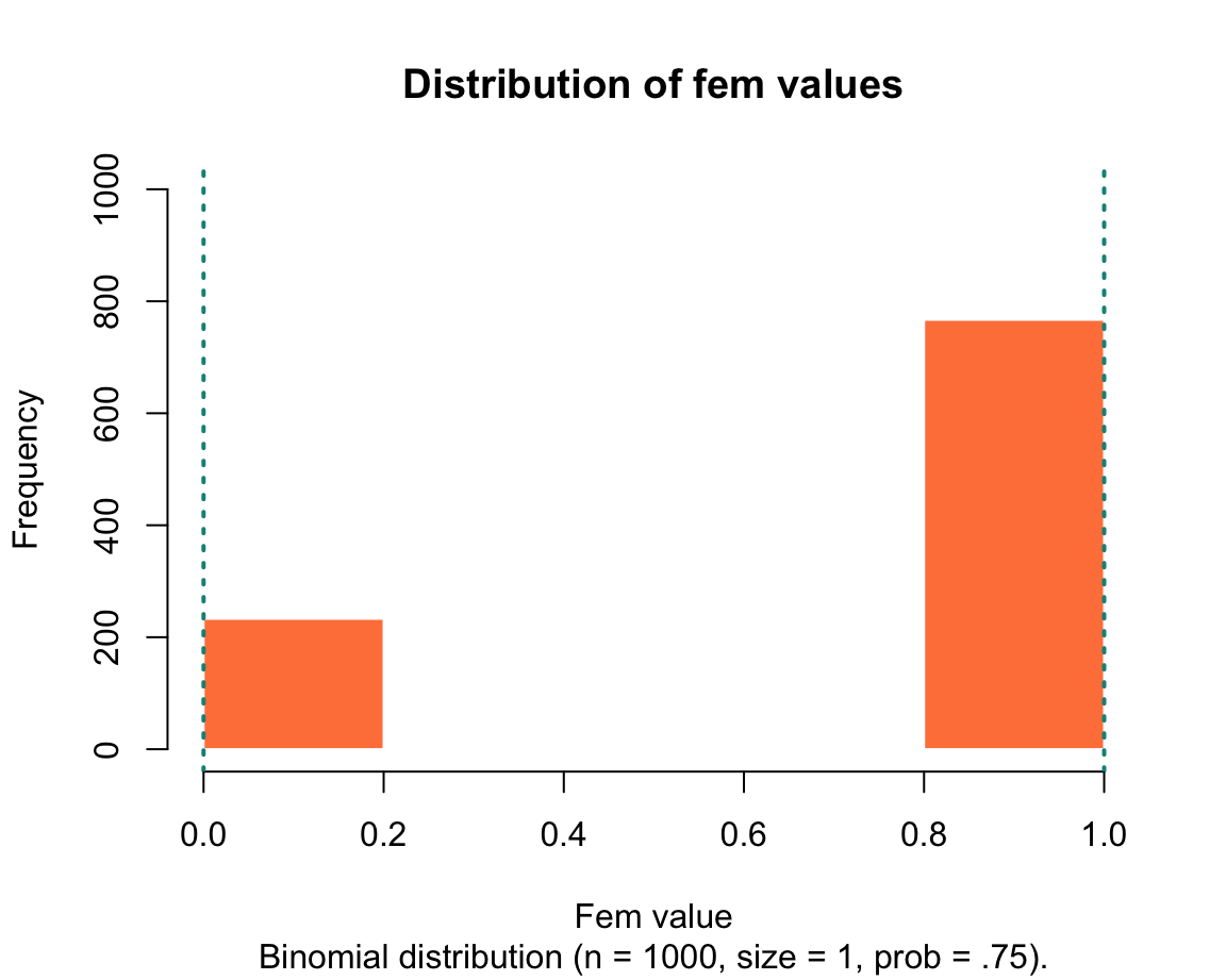
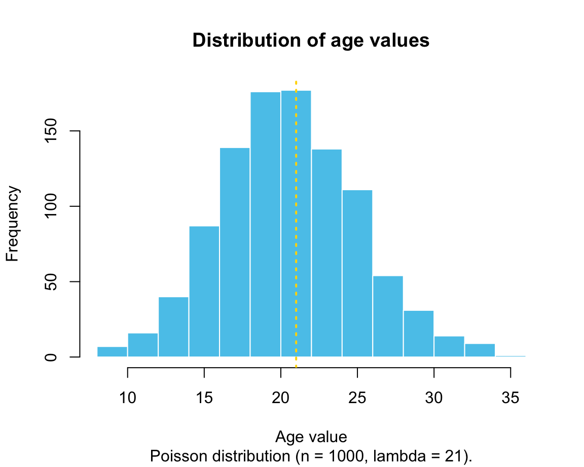
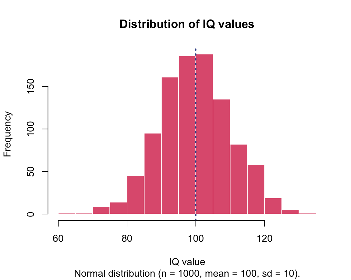
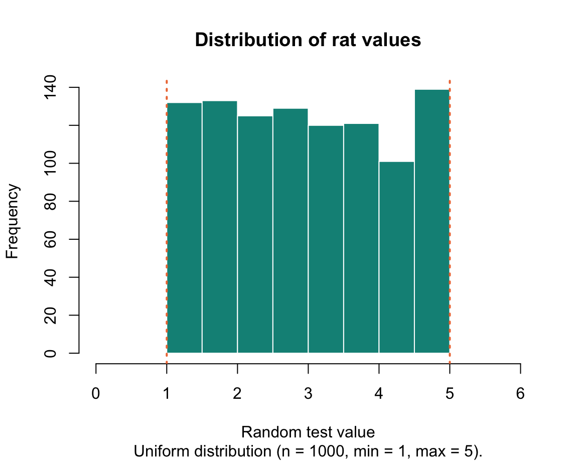
We will learn how to create these graphs in in Chapter 2 on Visualizing data.
Practice
Here are some tasks that practice random sampling:
- Selecting and sampling
LETTERS:
We have used the R object LETTERS in our practice of indexing/subsetting vectors above.
Combine subsetting and sampling to create a random vector of 10 elements, which are sampled (with replacement) from the letters “U” to “Z?”
Solution
# ?LETTERS
ix_U <- which(LETTERS == "U")
ix_Z <- which(LETTERS == "Z")
U_to_Z <- LETTERS[ix_U:ix_Z]
sample(x = U_to_Z, size = 10, replace = TRUE)- Creating sequences and samples:
Evaluate the following expressions and explain their results in terms of functions and their arguments (e.g., by looking up the documentation of ?seq and ?sample):
seq(0, 10, by = 3)
seq(0, 10, length.out = 10)

sample(c("A", "B", "C"), size = 3)
sample(c("A", "B", "C"), size = 4)
sample(c("A", "B", "C"), size = 5, replace = TRUE)- Flipping coins:
The ds4psy package contains a coin() function that lets you flip a coin once or repeatedly:
library(ds4psy)  # load the pkg

?coin() # show documentation- Explore the
coin()function and then try to achieve the same functionality by using thesample()function.
# Exploration:
coin()       # 1. default
coin(n = 5)  # 2. using the n argument
coin(n = 5, events = c("A", "B", "C"))  # 3. using both arguments
Solution
The three expressions using the coin() function can be re-created by using the sample() function with different arguments:
# 1. using only x and size arguments:
sample(x = c("H", "T"), size = 1)

# 2. sampling with replacement:
sample(x = c("H", "T"), size = 5, replace = TRUE)

# 3. sampling from a different set x:
sample(x = c("A", "B", "C"), size = 5, replace = TRUE) Note: As the coin() and sample() functions involve random sampling, reproducing the same functionality with different functions or calling the same function repeatedly does not always yield the same results (unless we fiddle with R’s random number generator).
1.6.5 Flow control
As we have seen when defining our first scalars or vectors (in Sections 1.3 and 1.4), it matters in which order we define objects. For instance, the following example first defines x as a (numeric) scalar 1, but then re-assigns x to a vector (of type integer) 1:10, before re-assigning x to a scalar (of type character) “oops”:
# Assigning x:
x <- 1
typeof(x)
#> [1] "double"

# Re-assigning x:
x <- 1:10
typeof(x)
#> [1] "integer"

# Re-assigning x:
x <- "oops"
typeof(x)
#> [1] "character"
Although this example may seem trivial, it illustrates two important points:
R executes code sequentially: The order in which code statements and assignments are evaluated matters.
Whenever changing an object by re-assigning it, any old content of it (and its type) is lost.
At first, this dependence on evaluation order and the “forgetfulness” of R may seem like a nuisance. However, both features actually have their benefits when programming algorithms that require distinctions between cases or repeated executions of code. We will discuss such cases in our introduction to Programming (see Chapters 11 and 12). But as it is likely that you will encounter examples of if-then statements or loops before getting to these chapters, we briefly mention 2 major ways in which we can control the flow of information here.
Conditionals
A conditional statement in R begins with the keyword if (in combination with some TEST that evaluates to either TRUE or FALSE) and a THEN part that is executed if the test evaluates to TRUE.
An optional keyword else and a corresponding ELSE part is executed if the test evaluates to FALSE.
The basic structures of a conditional test in R are the following:
if (TEST) {THEN}
if (TEST) {THEN} else {ELSE}
Notice that both if statements involve two different types of parentheses:
Whereas the TEST is enclosed in round parentheses (), the THEN and ELSE parts are enclosed in curly brackets {}.
Examples
The TEST part of a conditional is a statement that evaluates to a logical value of either TRUE or FALSE.
Thus, the most basic way for illustrating the selective nature if if and if else is the following:
x <- 10
if (TRUE)  { x <- 11 }
x
#> [1] 11
if (FALSE) { x <- 12 } else { x <- 13 }
x
#> [1] 13
In practice, the TEST part of a conditional will not just be a logical value, but some condition that is checked to determine whether to execute the THEN (or the ELSE) part of the conditional.
Using the current value of x (i.e., x = 13), try to predict the result of the following expressions:
y <- 1
if (x <= 10) { y <- 2 }
y
if (x == 13) { y <- 3 } else { y <- 4 }
y
if (x >  13) { y <- 5 } else { y <- 6 }
y
Hint: The three values of y are 1, 3, and 6.
A caveat: Users that come from other statistical software packages (like SAS or SPSS) often recode data by using scores of conditional statements. Although this is possible in R, its vector-based nature and the powers of (logical and numeric) indexing usually provide better solutions (see Section 11.3.7).
Practice
- Predict the final outcome of evaluating
yin the following code and then evaluate it to check your prediction:
y <- 11:22
if (length(y) > 11)  { x <- 30 } else { x <- 31 }
y <- "wow"
if (x < 31) { y <- x } else { y <- "!" }
y
Conditional statements are covered in greater detail in Chapter 11 on Functions (see Section 11.3). However, we will also see that the combination of vectorized data structures and indexing/subsetting (as introduced in Section 1.4.6) often allows us to avoid conditional statements in R (see Section 11.3.7).
Loops
Loops repeat particular lines of code as long as some criteria are met.
This can be achieved in several ways, but the most common form of loop is the for loop that increments an index or counter variable (often called i) within a pre-specified range.
The basic structure of a for loop in R is the following:
for (i in <LOOP_RANGE>) {

  <LOOP-BODY>

}
The code in <LOOP-BODY> is executed repeatedly — as often as indicated in <LOOP_RANGE>.
The variable i serves as a counter that indicates the current iteration of the loop.
Example
for (i in 1:10) {

  print(i)

}
#> [1] 1
#> [1] 2
#> [1] 3
#> [1] 4
#> [1] 5
#> [1] 6
#> [1] 7
#> [1] 8
#> [1] 9
#> [1] 10
Practice
- Predict the effects of the following loops and then evaluate them to check your prediction:
for (i in 4:9) {

  print(i^2)

}
for (i in 10:99) {
if (sqrt(i) %% 1 == 0) { print(i) }
}We will learn more about loops in our chapter on Iteration (Chapter 12).
This concludes our sneak preview on some more advanced aspects of R. Again, do not worry if some of them remain a bit fuzzy at this point — they will re-appear and be explained in greater detail later. Actually, most users of R solve pretty amazing tasks without being programmers or caring much about the details of the language. If you really want to understand the details of R, the Advanced R books by Hadley Wickham (2014a, 2019a) are excellent resources.
Let’s wrap up this chapter and check what we have learned by doing some exercises.
References
The default value of the argument
stringsAsFactorsused to beTRUEfor decades. As this caused much confusion, the default has now been changed. From R version 4.0.0 (released on 2020-04-24), the default isstringsAsFactors = FALSE. This shows that the R gods at https://cran.r-project.org/ are listening to user feedback, but you should not count on changes happening quickly.↩︎The recent switch from the default of
stringsAsFactors = TRUEtostringsAsFactors = FALSEactually teaches us an important lesson about R: Always be aware of defaults and try not to rely on them too much in your own code. Explicating the arguments used in our own functions will protect us from changes in implicit defaults. For background on R’sstringsAsFactorsdefault, see the post stringsAsFactors (by Kurt Hornik, on 2020-02-16) on the R developer blog.↩︎Internally, lists in R actually are vectors. However, rather than atomic vectors, lists are hierarchical or recursive vectors that can contain elements of multiple data types/modes and various shapes. (See Wickham, 2014a for details.)↩︎