1.7 Summary

This chapter provided a very brief introduction to R (R Core Team, 2021). After clarifying the terminology of R-related technologies, we distinguished functions (i.e., objects that do things) from data objects (i.e., objects that are being defined and computed). Data objects are distinguished by their data type and shape:
The most important types of data are truth values (of type
logical), numbers (integerordouble), text (character), and time-based data (with types for dates and times).The most important shapes of data are vectors (i.e., linear and homogeneous data structures that are characterized by their length and type) and rectangular tables (i.e., two-dimensional data structures that can contain heterogeneous data, with each column being a vector).
Table 1.5 merely repeats the overview of data structures from Section 1.2.1:
| Dimensions: | Homogeneous data types: | Heterogeneous data types: |
|---|---|---|
| 1D | atomic vectors: vector |
list |
| 2D | matrix |
rectangular tables: data.frame/tibble |
| nD | array/table |
From a user’s perspective, the two most important shape-type combinations are atomic vectors and rectangular tables, but is good to know that the latter (e.g., objects of type data.frame or tibble) are implemented as lists.
In the rest of this chapter, we showed how to create new data objects (i.e., vectors, matrices, and data frames) and illustrated basic functions to access, check, manipulate, and tranform them (e.g., by numerical or logical indexing). Finally, and only to familiarize us with some additional concepts, we briefly sketched some advanced issues — like factors, lists, random sampling, conditionals, and loops — in Section 1.6.
After working through this chapter, you are able to:
- explain why R is and is not like a Swiss knife;
- categorize R objects into data vs. functions;
- distinguish between different shapes (e.g., scalars, vectors, rectangles) and types (e.g., numeric, character, logical) of data;
- create and change R objects (by assignment);
- apply arithmetic functions to numeric data objects;
- create and modify vectors and rectangular tables of data;
- select elements from vectors and rectangular tables of data (by indexing);
- recognize some more advanced issues (e.g., factors, lists, random sampling, conditionals, and loops).
If you made it to this point, you can congratulate yourself. As this chapter contains the essentials of R, successfully working through it is quite an achievement. However, as all of R cannot be covered in a single chapter, the mystery and scope of R extend far beyond this introduction. At this point, it may be a good idea to take a look at the RStudio cheatsheet on Base R (contributed by Mhairi McNeill) to check which concepts and commands you are now familiar with and which others you may still discover in the future:
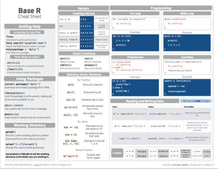
Figure 1.4: Base R summary from RStudio cheatsheets.
The following chapters introduce new tasks and tools for transforming, visualizing, and understanding data. Some of these chapters adopt a tidyverse (Wickham et al., 2019) perspective to apply and use R. But as the R packages of the tidyverse (Wickham, 2019c) are embedded in the larger ecosystem of R, we also provide background information on base R functions that can solve the same or related tasks.
But before we continue, let’s seize the opportunity to test our knowledge and skills on base R concepts and commands by completing the following exercises.