A.1 Solutions (01)

Here are the solutions to the exercises on Chapter 1: Basic R concepts and commands (Section 1.8).
A.1.1 Exercise 1
Creating and changing R objects
Our first exercise (on Section 1.2) begins by cleaning up our current working environment and then defines, evaluates, and changes some R objects.
Cleaning up: Check the Environment tab of RStudio to see which objects are currently defined to which values (after working through this chapter). Then run
rm(list = ls())and explain what happens (e.g., by reading the documentation of?rm).Creating R objects: Create some new R objects by evaluating the following assignment expressions:
a <- 100
b <- 2
d <- "weird"
e <- TRUE
o <- FALSE
O <- 5- Evaluating and changing R objects: Given this set of new R objects, evaluate the following expressions and explain their results (correcting for any errors that may occur):
a
b
c <- a + a
a + a == c

!!a
as.logical(a)

sqrt(b)
sqrt(b)^b
sqrt(b)^b == b

o / O
o / O / 0

o <- "ene mene mu"
o / O / 0

o <- FALSE
o / O / 0

a + b + C

sum(a, b) - sum(a + b)

b:a

i <- i + 1

nchar(d) - length(d)

e
e + e + !!e
e <- stuff
paste(d, e)
Solution
- ad 1. Cleaning up: Removing all objects in the current working environment:
rm(list = ls()) # remove ALL objects (without warning)Note that running rm(list = ls()) will issue no warning, so we must only ever use this when we no longer need the objects currently defined (i.e., when we want to start with a clean slate).
- ad 2. Creating R objects: Given this set of new R objects, evaluate the following expressions and explain their results (correcting for any errors that may occur):
a <- 100
b <- 2
d <- "weird"
e <- TRUE
o <- FALSE # OR
# o <- "ene mene mu"
O <- 5- ad 3. Evaluating and changing R objects: The following code chunk evaluates the expressions and contains explanations and corrections (as comments):
# Note: The following assume the object definitions from above.
a  # 100
#> [1] 100
b  # 2
#> [1] 2
c <- a + a  # c created/defined as a + a
a + a == c  # TRUE, as both evaluate to 200
#> [1] TRUE

!!a            # TRUE, as
#> [1] TRUE
as.logical(a)  # TRUE
#> [1] TRUE

# Note:
as.logical(1)  # a number is interpreted as TRUE,
#> [1] TRUE
as.logical(0)  # but 0 is interpreted as FALSE
#> [1] FALSE

sqrt(b)         # see ?sqrt
#> [1] 1.414214
sqrt(b)^b       # same as b = 2 (as it should)
#> [1] 2
sqrt(b)^b == b  # Why FALSE?
#> [1] FALSE

# Hint: Compute the difference sqrt(2)^2 - 2
sqrt(b)^b - b   # is not 0, but some very small number.
#> [1] 4.440892e-16

# Using objects o and O (from above):
o / O       # 0
#> [1] 0
o / O / 0   # NaN (not a number)
#> [1] NaN
# If o is set to "ene mene mu":
o <- "ene mene mu"
o / O / 0   # Error, as o is non-numeric.
#> Error in o/O: non-numeric argument to binary operator
# If o is set o FALSE:
o <- FALSE
o / O / 0   # NaN, as we're dividing 0/0 again.
#> [1] NaN
# Correction: Set o to some number:
o <- 1
0 / (o * O)  # works
#> [1] 0
0 / (o * 0)  # NaN, due to division of 0/0.
#> [1] NaN

a + b + C   # are all objects defined?
#> Error in a + b + C: non-numeric argument to binary operator
# C is defined as? some function (see ?C for details)
# Correction: Set C to some number:
C <- 1
a + b + C  # evaluates to 103
#> [1] 103

sum(a, b) - sum(a + b)  # 0
#> [1] 0
# Explanation:
sum(a, b)   # 102
#> [1] 102
sum(a + b)  # 102
#> [1] 102

b:a  # does NOT divide b by a!
#>  [1]  2  3  4  5  6  7  8  9 10 11 12 13 14 15 16 17 18 19 20 21 22 23 24 25 26
#> [26] 27 28 29 30 31 32 33 34 35 36 37 38 39 40 41 42 43 44 45 46 47 48 49 50 51
#> [51] 52 53 54 55 56 57 58 59 60 61 62 63 64 65 66 67 68 69 70 71 72 73 74 75 76
#>  [ reached getOption("max.print") -- omitted 24 entries ]
# Explanation: b:a creates a vector of integers from b = 2 to a = 100:
length(b:a)  # 99 elements
#> [1] 99

i <- i + 1  # increment i by 1
#> Error in eval(expr, envir, enclos): object 'i' not found
# Error: i is not defined.
# Correction: Set i to some number:
i <- 1
i <- i + 1  # works:
i           # 2
#> [1] 2

nchar(d) - length(d)  # returns 4
#> [1] 4
# Explanation:
d          # d is set to "weird"
#> [1] "weird"
nchar(d)   # 5 characters
#> [1] 5
length(d)  # 1 element (in character vector, scalar)
#> [1] 1

e  # TRUE
#> [1] TRUE
e + e + !!e  # 1 + 1 + 1 = 3
#> [1] 3

e <- stuff    # Error: stuff is not defined.
#> Error in eval(expr, envir, enclos): object 'stuff' not found
# Correction:
e <- "stuff"  # define e as a character (text) object
paste(d, e)   # works: "weird stuff"
#> [1] "weird stuff"
A.1.2 Exercise 2
Fun with plot functions
In Section 1.2.5, we explored the plot_fn() function of the ds4psy package to discover the meaning of its arguments.
In this exercise, you will explore another function of the same package.
- Assume the perspective of an empirical scientist to explore and decipher the arguments of the
plot_fun()function in a similar fashion.
library(ds4psy)  # loads the package

plot_fun()  # calls the function (with default arguments)
Hint: Solving this task essentially means to answer the question “What does this argument do?”
for each argument (i.e., the lowercase letters from a to f, and c1 and c2).
Solution
The documentation of plot_fun() (available via ?plot_fun()) shows the following list of arguments:
aA (natural) number. Default:a = NA.bA Boolean value. Default:b = TRUE.cA Boolean value. Default:c = TRUE.dA (decimal) number. Default:d = 1.0.eA Boolean value. Default:e = FALSE.fA Boolean value. Default:f = FALSE.gA Boolean value. Default:g = FALSE.c1A color palette (e.g., as a vector). Default:c1 = c(rev(pal_seeblau), "white", pal_grau, "black", Bordeaux).c2A color (e.g., as a character). Default:c2 = "black".
The plot_fun() function of the ds4psy is a simplified and deliberately obscured version of the plot_tiles() function.
See the documentation of the latter (via ?plot_tiles()) to obtain the documentation of its arguments.
- Use your exploration of
plot_fun()to reconstruct the command that creates the following plots:
Hint: Check the documentation of plot_fun() (e.g., for color information).
Solution
plot_fun(a = 5, d = 4, e = TRUE, c2 = "white")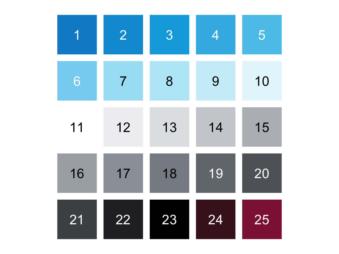
plot_fun(a = 4, c = FALSE, f = TRUE, g = TRUE, c1 = c("steelblue", "white", "firebrick"))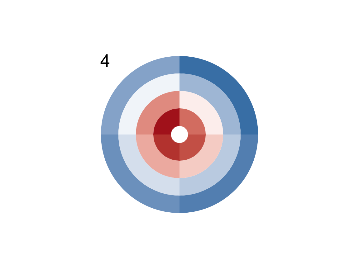
A.1.3 Exercise 3
Dice sampling
In Section 1.6.4, we explored the coin() function of the ds4psy package and mimicked its functionality by the sample() function. In this exercise, we will explore the dice() and dice_2() functions of the same package.
- Explore the
dice()function (of the ds4psy package) by first calling it a few times (with and without arguments). Then study its documentation (by calling?dice()).
Solution
# Exploring the function:
dice()
#> [1] 6
dice(n = 10)
#>  [1] 6 6 3 5 6 2 5 4 6 1
dice(n = 10, events = 6:9)
#>  [1] 9 8 6 6 6 7 8 8 8 8
dice(n = 10, events = c("X", "Y", "Z"))
#>  [1] "Z" "Y" "X" "Z" "X" "Y" "Y" "Y" "Z" "Y"

?dice() # show documentation- Explore the
dice_2()function (of the ds4psy package) by first calling it a few times (with and without arguments). Then study its documentation (by calling?dice_2()).
What are the differences between thedice()anddice_2()functions?
Solution
# Exploring the function:
dice_2()
#> [1] 1
dice_2(n = 10)
#>  [1] 6 1 1 6 4 2 5 5 6 5
dice_2(n = 10, sides = 6)
#>  [1] 2 2 5 2 4 5 4 5 5 4
dice_2(10, sides = c("X", "Y", "Z"))
#>  [1] "Y" "Y" "Y" "Z" "X" "X" "Y" "Z" "Y" "Z"
Answer:
An obvious difference between the
dice()anddice_2()functions is thatdice()uses an argumentevents(which is typically set to a vector) whereasdice_2()uses an argumentsides(which is typically set to a number). However, both arguments can be set to an arbitrary vector of events.Discovering a less obvious difference requires a more thorough investigation: As both functions include random sampling, we need to call them not just a few times, but many times to examine their validity.
Compare what happens when we call both functions N times for some pretty large value of N:
N <- 6 * 100000

# Exploring dice():
min(dice(N))   # min = 1
#> [1] 1
max(dice(N))   # max = 6
#> [1] 6
mean(dice(N))  # mean --> 3.50 (i.e., (min + max)/2)
#> [1] 3.500215

# Exploring dice_2():
min(dice_2(N))   # min = 1
#> [1] 1
max(dice_2(N))   # max = 6
#> [1] 6
mean(dice_2(N))  # mean > 3.50 !!!
#> [1] 3.535108
Thus, whereas both functions seem to have the same minimum and maximum, dice_2() seems to have a higher mean value of than dice_2().
The reason for this becomes obvious when we cross-tabulate the outcomes of both functions:
table(dice(N))
#>
#>      1      2      3      4      5      6
#>  99366 100480  99504 100011 100260 100379
table(dice_2(N))
#>
#>      1      2      3      4      5      6
#>  98669  98468  98587  98150  98771 107355
Thus, dice_2() is biased — by default, it throws more outcomes of 6 than any other number.
Bonus task: Use the base R function
sample()to sample from the numbers1:6so thatsample()yields a fair dice in which all six numbers occur equally often, andsample()yields a biased dice in which the value6occurs twice as often as any other number.
Hint: The prob argument of sample() can be set to a vector of probability values
(i.e., as many values as length(x) that should sum up to a total value of 1).
Solution
a. Fair dice:
# (a) Sampling 10 times:
sample(x = 1:6, size = 10, replace = TRUE)
#>  [1] 3 2 3 5 6 3 3 4 6 3

# Sampling N times:
N <- 100000
table(sample(x = 1:6, size = N, replace = TRUE))
#>
#>     1     2     3     4     5     6
#> 16583 16758 16667 16624 16631 16737

# Generalization: Using objects to set x and prob:
events <- 1:6
n_events <- length(events)
# Create vector of n_events equal probability values:
p_events <- rep(1/n_events, n_events)

# Checks:
p_events
#> [1] 0.1666667 0.1666667 0.1666667 0.1666667 0.1666667 0.1666667
sum(p_events)
#> [1] 1

# Sampling N times with prob = p_events:
table(sample(x = events, size = N, replace = TRUE, prob = p_events))
#>
#>     1     2     3     4     5     6
#> 16462 16885 16833 16454 16796 16570
b. Biased dice:
To create the biased dice, we need to define a vector of probability values
in which the the final of n_events values is twice as large
as the values of the preceding n_events - 1 elements:
# (b) Create vector of biased probability values:
p_biased <- c(1/7, 1/7, 1/7, 1/7, 1/7,  # first 5 elements
              2/7)                      # 6th element twice as large
p_biased
#> [1] 0.1428571 0.1428571 0.1428571 0.1428571 0.1428571 0.2857143
sum(p_biased)
#> [1] 1

# More general solution (based on n_events):
p_biased <- c(rep(1/(n_events + 1), n_events - 1), 2/(n_events + 1))

# Checks:
p_biased
#> [1] 0.1428571 0.1428571 0.1428571 0.1428571 0.1428571 0.2857143
sum(p_biased)
#> [1] 1

# Sampling N times with prob = p_biased:
table(sample(x = 1:6, size = N, replace = TRUE, prob = p_biased))
#>
#>     1     2     3     4     5     6
#> 14360 14396 14243 14346 14196 28459
A.1.4 Exercise 4
Cumulative savings
With only a little knowledge of R you can perform quite fancy financial arithmetic.
Assume that you have won an amount a of EUR 1000 and are considering to deposit this amount into a new bank account that offers an annual interest rate int of 0.1%.
How much would your account be worth after waiting for \(n = 2\) full years?
What would be the total value of your money after \(n = 2\) full years if the annual inflation rate
infis 2%?What would be the results to 1. and 2. if you waited for \(n = 10\) years?
Answer these questions by defining well-named objects and performing simple arithmetic computations on them.
Note:
Solving these tasks in R requires defining some numeric objects (e.g., a, int, and inf) and performing arithmetic computations with them (e.g., using +, *, ^, with appropriate parentheses).
Do not worry if you find these tasks difficult at this point — we will revisit them later.
In Exercise 6 of Chapter 12: Iteration, we will use loops and functions to solve such tasks in a more general fashion.
Solution
# Definitions:
a_0 <- 1000     # initial amount of savings (year 0)
int  <- .1/100  # interest rate (annual)
inf <- 2/100    # inflation rate (annual)
n <- 2          # number of years

## 1. Savings with interest: -----

# 1a. In 2 steps:
a_1 <- a_0 + (a_0 * int)  # after 1 year
a_1
#> [1] 1001

a_2 <- a_1 + (a_1 * int)  # after 2 years
a_2
#> [1] 1002.001

# 1b. Both in 1 step:
a_0 * (1 + int)^n
#> [1] 1002.001


# 2. Also accounting for inflation: -----
total <- a_0 * (1 + int - inf)^n
total
#> [1] 962.361

# 3. Different numbers of years:
n <- 10

# Use formulas from 1b and 2:
a_0 * (1 + int)^n        # interest only
#> [1] 1010.045
a_0 * (1 + int - inf)^n  # interest + inflation
#> [1] 825.4487
Note: Do not worry if you find this task difficult at this point — we will revisit it later. In Exercise 6 of Chapter 12: Iteration, we will use loops and functions to solve it in a more general fashion.
A.1.5 Exercise 5
Vector arithmetic
When introducing arithmetic functions above, we showed that they can be used with numeric scalars (i.e., numeric objects with a length of 1).
Demonstrate that the same arithmetic functions also work with two numeric vectors
xandy(of the same length).What happens when
xandyhave different lengths?
Hint: Define some numeric vectors and use them as arguments of various arithmetic functions. To better understand the behavior in 2., look up the term “recycling” in the context of R vectors.
Solution
Arithmetic with vectors, rather than scalars:
## 1. Arithmetic with vectors of the same length:
x <- c(2, 4, 6)
y <- c(1, 2, 3)

+ x     # keeping sign
#> [1] 2 4 6
- y     # reversing sign
#> [1] -1 -2 -3
x + y   # addition
#> [1] 3 6 9
x - y   # subtraction
#> [1] 1 2 3
x * y   # multiplication
#> [1]  2  8 18
x / y   # division
#> [1] 2 2 2
x ^ y   # exponentiation
#> [1]   2  16 216
x %/% y # integer division
#> [1] 2 2 2
x %% y  # remainder of integer division (x mod y)
#> [1] 0 0 0
When vectors have different lengths, the shorter one is recycled to the length of the longer one (and a Warning is issued). The result of vector arithmetic involving multiple vectors is a vector with as many elements as the longest vector:
## 2. Arithmetic with vectors of different lengths:
x <- c(2, 4, 6)
y <- c(1, 2)

+ x     # keeping sign
#> [1] 2 4 6
- y     # reversing sign
#> [1] -1 -2
x + y   # addition
#> [1] 3 6 7
x - y   # subtraction
#> [1] 1 2 5
x * y   # multiplication
#> [1] 2 8 6
x / y   # division
#> [1] 2 2 6
x ^ y   # exponentiation
#> [1]  2 16  6
x %/% y # integer division
#> [1] 2 2 6
x %% y  # remainder of integer division (x mod y)
#> [1] 0 0 0
The recycling behavior of vectors (in the context of arithmetic functions) generalizes to more than two vectors:
## Generalize to 3 vectors:
x <- c(1)
y <- c(1, 2)
z <- c(1, 2, 3)

x + y + z  # => 3 5 5 + Warning
#> [1] 3 5 5

# Explanation: Due to recycling of x and y to the length of z,
# R actually computes:
# c(1, 1, 1) + c(1, 2, 1) + c(1, 2, 3)
However, note that recycling does not automatically generalize to all R functions:
x <- 1:10
y <- c(-1, 1)

# Recycling y:
x * y
#>  [1] -1  2 -3  4 -5  6 -7  8 -9 10
x + y
#>  [1]  0  3  2  5  4  7  6  9  8 11

# Not recycling y:
data.frame(x, y)
#>     x  y
#> 1   1 -1
#> 2   2  1
#> 3   3 -1
#> 4   4  1
#> 5   5 -1
#> 6   6  1
#> 7   7 -1
#> 8   8  1
#> 9   9 -1
#> 10 10  1
A.1.6 Exercise 6
Cryptic arithmetic
Predict the result of the arithmetic expression x %/% y * y + x %% y.
Then test your prediction by assigning some positive number(s) to x and to y and evaluating the expression.
Finally, explain why the result occurs.
Solution
## Note: The given expression
x %/% y * y + x %% y
#>  [1]  1  2  3  4  5  6  7  8  9 10
# is identical to:
((x %/% y) * y) + (x %% y)
#>  [1]  1  2  3  4  5  6  7  8  9 10

## Prediction: The expression
x %/% y * y + x %% y  # will evaluate to x.
#>  [1]  1  2  3  4  5  6  7  8  9 10

## Testing the prediction:
x <- 4711
y <- 1307

((x %/% y) * y) + (x %% y) == x  # prediction is TRUE
#> [1] TRUE

## Explanation:
x %/% y      # yields the integer part of x/y
#> [1] 3
x %/% y * y  # multiplies this integer part by y
#> [1] 3921
x %% y       # yields the remainder of integer division
#> [1] 790

# => The sum
(x %/% y * y) + (x %% y)
#> [1] 4711
# yields x.
Note that evaluating expression x %/% y * y + x %% y still yields x when x and y are numeric vectors with multiple elements.
Demonstration:
x <- c(2, 4, 6, 8)
y <- c(1/3, pi)

(x %/% y * y) + (x %% y)
#> [1] 2 4 6 8
When the vectors x and y have different lengths, the shorter vector is recycled to match the length of the longer one.
A.1.7 Exercise 7
Survey age
Assume the following definitions for a survey:
A person with an age from 1 to 17 years is classified as a minor;
a person with an age from 18 to 64 years is classified as an adult;
a person with an age from 65 to 99 years is classified as a senior.
Generate a vector with 100 random samples that specifies the age of 100 people (in years), but contains exactly 20 minors, 50 adults, and 30 seniors.
Now use some functions on your age vector to answer the following questions:
What is the average (mean), minimum, and maximum age in this sample?
How many people are younger than 25 years?
What is the average (mean) age of people older than 50 years?
How many people have a round age (i.e., an age that is divisible by 10)? What is their mean age?
Solution
set.seed(42) # for replicable randomness

# Creating 3 groups:
minor_range  <-  1:17
adult_range  <- 18:64
senior_range <- 64:99

# Creating 3 vectors (1 for each sub-group):
minors  <- sample(minor_range, 20, replace = TRUE)
adults  <- sample(adult_range, 50, replace = TRUE)
seniors <- sample(senior_range, 30, replace = TRUE)

# Combining 3 vectors into 1:
age <- c(minors, adults, seniors)
age
#>  [1] 17  5  1 10  4 17 15  7  4  5 14 15  3  9  4  5 13  5  2  8 20 50 59 41 47
#> [26] 60 32 39 25 53 21 39 35 62 45 22 21 51 52 41 40 43 23 23 19 20 38 19 55 27
#> [51] 57 22 50 56 53 62 59 26 46 29 37 26 60 52 46 33 54 45 63 22 91 65 81 87 81
#>  [ reached getOption("max.print") -- omitted 25 entries ]

# Checks:
length(age)
#> [1] 100
min(age)
#> [1] 1
max(age)
#> [1] 99
range(age)
#> [1]  1 99
mean(age)
#> [1] 46.45

# Using indexing:
# How many people are younger than 25 years?
length(age[age < 25])
#> [1] 31

# What is the average (mean) age of people older than 50 years?
mean(age[age > 50])
#> [1] 73.26087

# Round age:
round_ages <- age[age %% 10 == 0]
length(round_ages)
#> [1] 10
mean(round_ages)
#> [1] 48
A.1.8 Exercise 8
Exploring participant data
Explore the participant information of p_info (Woodworth, O’Brien-Malone, Diamond, & Schüz, 2018) by describing each of its variables:
How many individuals are contained in the dataset?
What percentage of them is female (i.e., has a
sexvalue of 1)?How many participants were in one of the 3 treatment groups (i.e., have an
interventionvalue of 1, 2, or 3)?What is the participants’ mean education level? What percentage has a university degree (i.e., an
educvalue of at least 4)?What is the age range (
mintomax) of participants? What is the average (mean and median) age?Describe the range of
incomelevels present in this sample of participants. What percentage of participants self-identifies as a below-average income (i.e., anincomevalue of 1)?Bonus task: The variables of
p_infoare stored as numeric variables, but some could also be factors.Which of the variables could or should be turned into factors?
It seems thatintervention,sex,educandincomecould/should be turned into factors.Recode some variables as factors (by consulting the codebook in Section 1.6.1).
Verify that the recoded factors correspond to the original variables.
Hint: The p_info data was defined and described above (in Section 1.6.1).
As it is also included as a tibble posPsy_p_info in the ds4psy package, it can be obtained by (re-)assigning:
p_info <- ds4psy::posPsy_p_infoSolution
Here are the solutions to Questions 1 to 6:
# Load data:
# (a) from the ds4psy package:
library(ds4psy)
p_info <- ds4psy::posPsy_p_info  # copy data

# (b) from file (stored online):
# p_info <- readr::read_csv(file = "http://rpository.com/ds4psy/data/posPsy_participants.csv")
# p_info

## 1. Number of participants: -----
n_total <- nrow(p_info)
n_total
#> [1] 295

## 2. How many female participants? -----
n_female <- length(p_info$sex[p_info$sex == 1])
n_female
#> [1] 251
n_female <- sum(p_info$sex == 1)     # alternative solution

pc_female <- n_female/n_total * 100  # compute percentage
pc_female
#> [1] 85.08475

## 3. How many participants are in an intervention group? -----
range(p_info$intervention)
#> [1] 1 4
hist(p_info$intervention, col = Seeblau)  # plots a histogram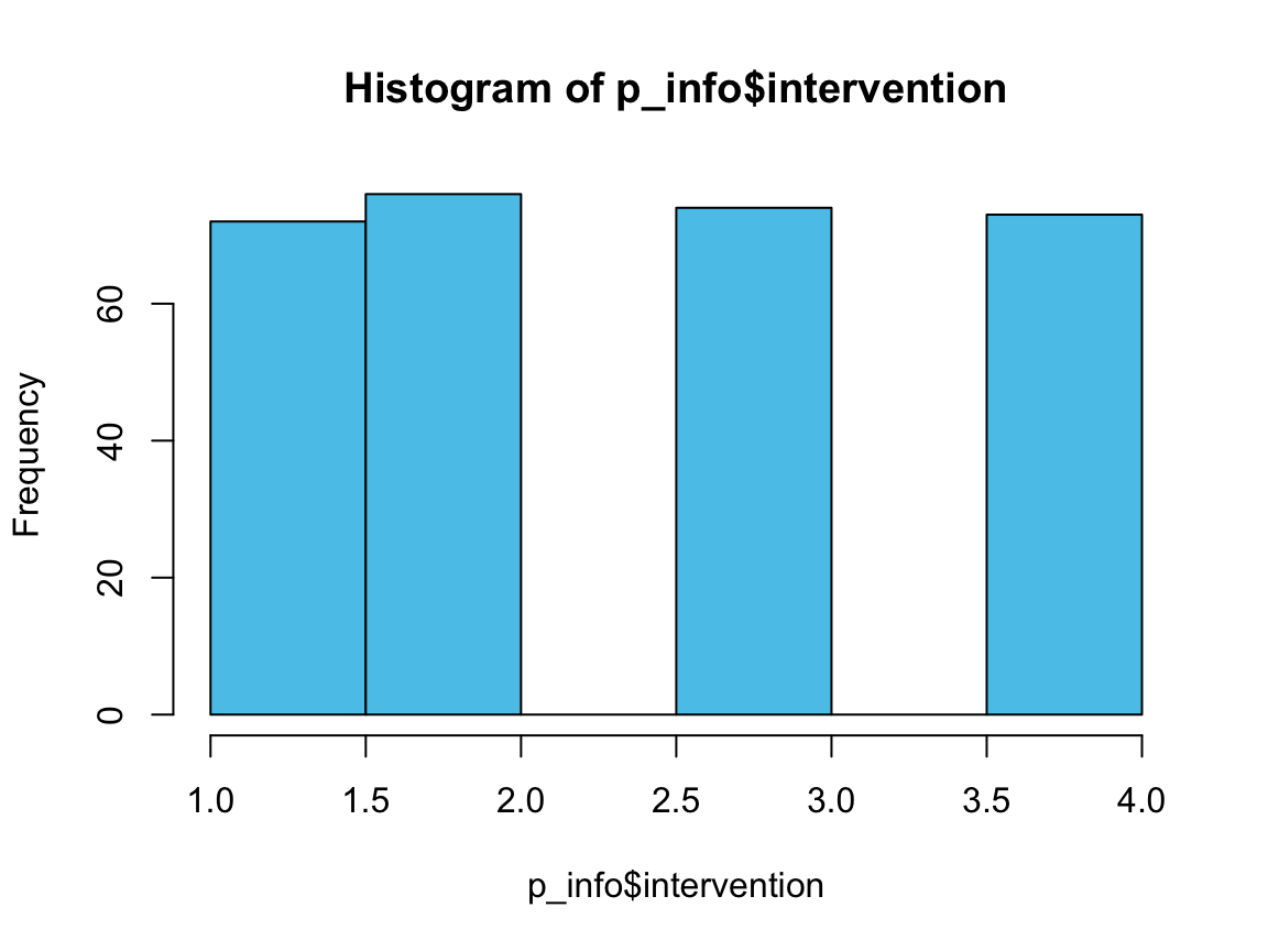
n_i1 <- sum(p_info$intervention == 1)
n_i2 <- sum(p_info$intervention == 2)
n_i3 <- sum(p_info$intervention == 3)
n_i4 <- sum(p_info$intervention == 4)

n_treat <- n_i1 + n_i2 + n_i3
n_treat
#> [1] 222

# Check: All participants NOT in control group 4:
n_treat == (n_total - n_i4)
#> [1] TRUE

## 4. Education level: -----
hist(p_info$educ, col = Bordeaux)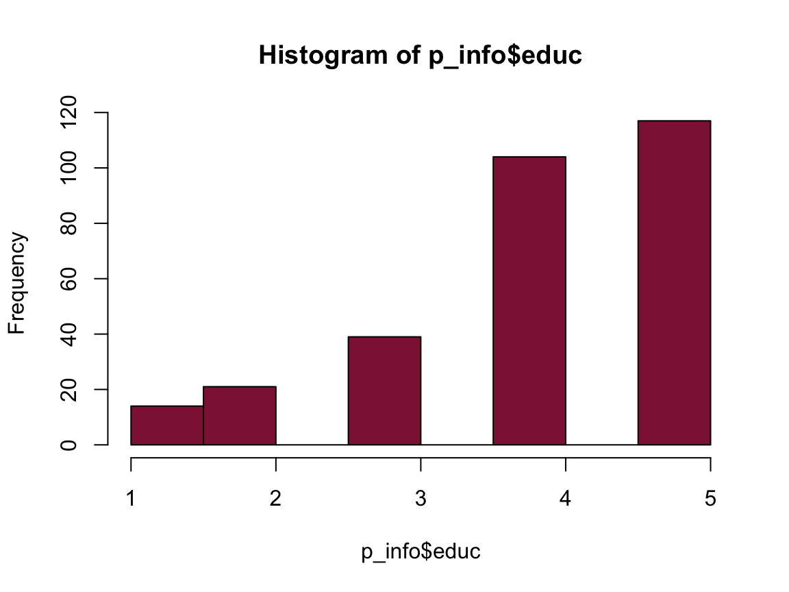
mean(p_info$educ)
#> [1] 3.979661
n_educ_uni <- sum(p_info$educ >= 4)

pc_educ_uni <- n_educ_uni/n_total * 100
pc_educ_uni
#> [1] 74.91525

## 5. Age: -----
hist(p_info$age, col = Seegruen)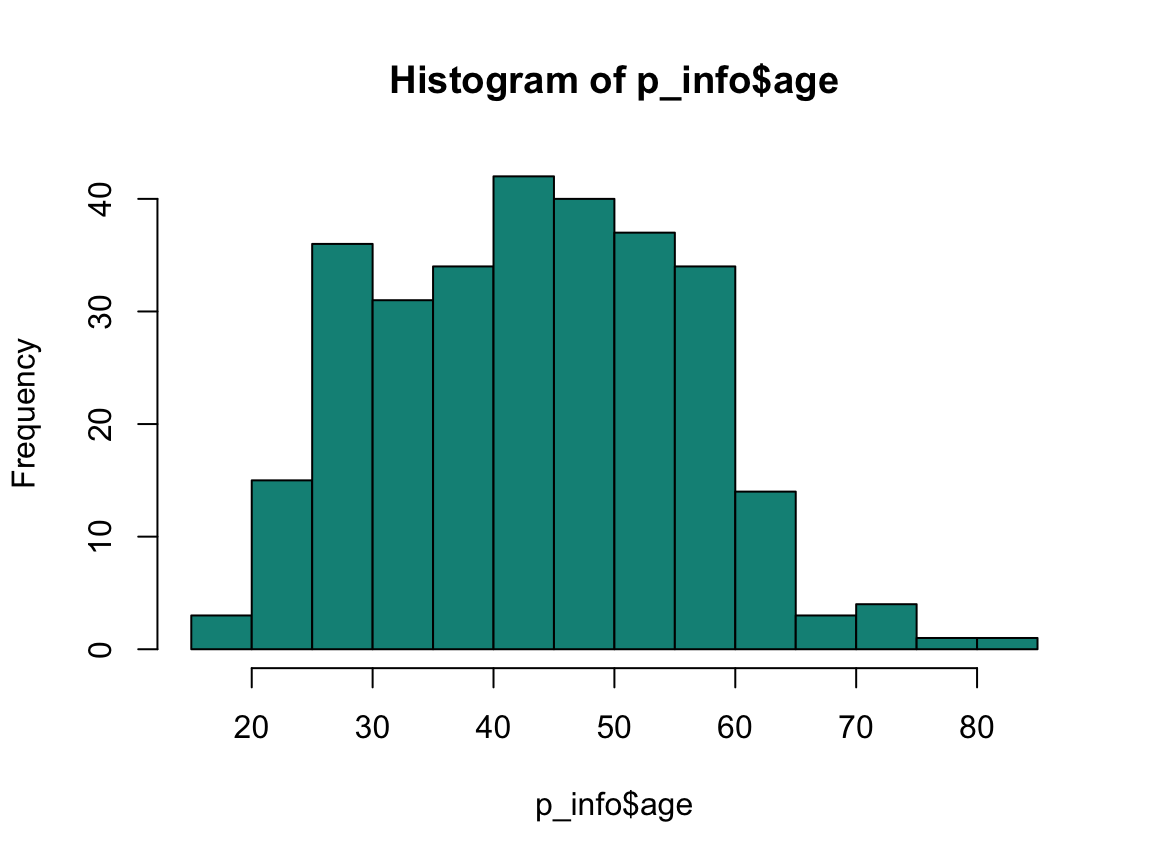
range(p_info$age)
#> [1] 18 83
mean(p_info$age)
#> [1] 43.75932
median(p_info$age)
#> [1] 44

## 6. Income: -----
hist(p_info$income, col = Pinky)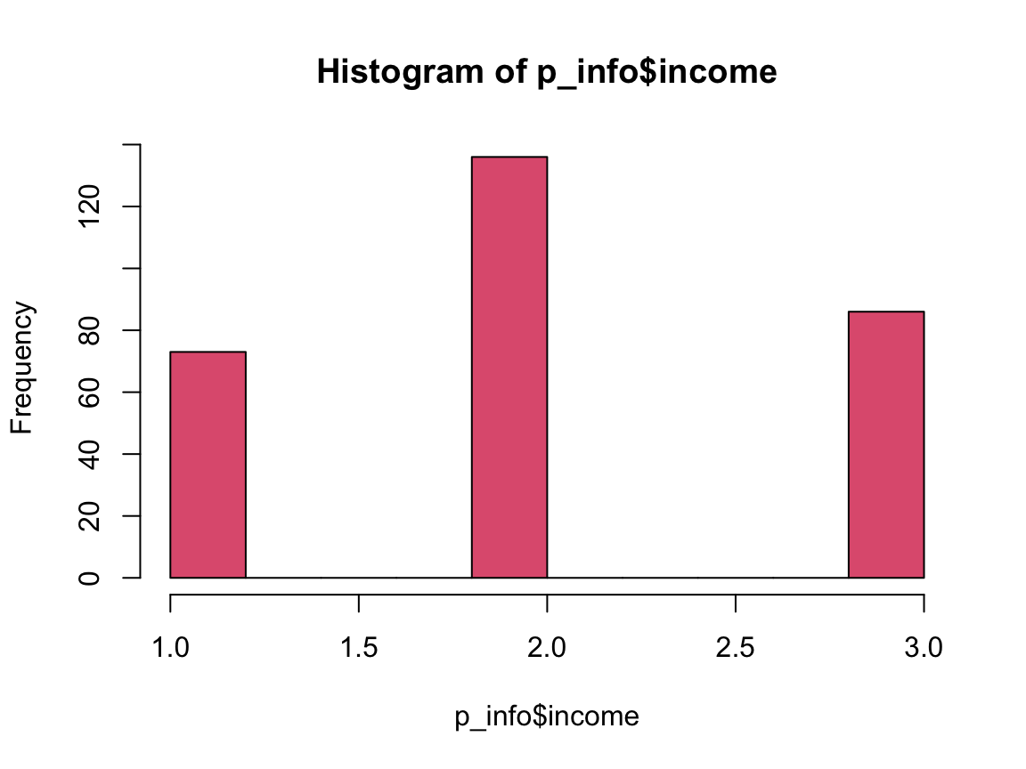
n_income_low <- sum(p_info$income < 2)
pc_income_low <- n_income_low/n_total * 100
pc_income_low
#> [1] 24.74576
Answers to Questions 1 to 6 of Exercise 8:
The
p_infodata contains 295 individuals.85.08% of the participants are female.
222 of the participants are in one of the three treatment groups.
74.92% of the participants have a university degree.
Participant’s age values range from 18 to 83 years. Their mean age is 43.76 years, their median age is 44 years.
24.75% of the participants state that their income is below average.
Solution
Bonus task: The variables of
p_infoare stored as numeric variables, but some could also be factors.Which of the variables could or should be turned into factors?
It seems thatintervention,sex,educandincomecould/should be turned into factors.Recode some variables as factors (by consulting the codebook in Section 1.6.1).
Verify that the recoded factors correspond to the original variables.
For recoding the variables as factors, we copy the data of p_info into an object p_data (to allow comparing our results with the original data later). Alternatively, we could also define the factors as new variables of p_info and later compare these new variables with the original ones.
p_info <- ds4psy::posPsy_p_info  # (re-)load data from ds4psy package
p_data <- p_info  # copy data
p_data  # => Numeric variables, rather than factors.
#> # A tibble: 295 × 6
#>       id intervention   sex   age  educ income
#>    <dbl>        <dbl> <dbl> <dbl> <dbl>  <dbl>
#>  1     1            4     2    35     5      3
#>  2     2            1     1    59     1      1
#>  3     3            4     1    51     4      3
#>  4     4            3     1    50     5      2
#>  5     5            2     2    58     5      2
#>  6     6            1     1    31     5      1
#>  7     7            3     1    44     5      2
#>  8     8            2     1    57     4      2
#>  9     9            1     1    36     4      3
#> 10    10            2     1    45     4      3
#> # … with 285 more rows

# Recoding (based on the codebook):

# Variable `intervention` with 4 levels:
# - 1 = “Using signature strengths”,
# - 2 = “Three good things”,
# - 3 = “Gratitude visit”,
# - 4 = “Recording early memories” (control condition).
p_data$intervention <- factor(p_data$intervention,
                              levels = c(1, 2, 3, 4),
                              labels = c("1. signature", "2. good things",
                                         "3. gratitude", "4. memories (control)"))

# Check:
summary(p_data$intervention)
#>          1. signature        2. good things          3. gratitude
#>                    72                    76                    74
#> 4. memories (control)
#>                    73

# Variable `sex` with 2 levels:
# - 1 = female,
# - 2 = male.
p_data$sex <- factor(p_data$sex, levels = c(1, 2), labels = c("female", "male"))

# Check:
summary(p_data$sex)
#> female   male
#>    251     44

# Variable `educ` with 5 levels:
#     - 1 = Less than Year 12,
#     - 2 = Year 12,
#     - 3 = Vocational training,
#     - 4 = Bachelor’s degree,
#     - 5 = Postgraduate degree.
p_data$educ <- factor(p_data$educ, levels = 1:5)

# Check:
summary(p_data$educ)
#>   1   2   3   4   5
#>  14  21  39 104 117

# Variable `income` with 3 levels:
#     - 1 = below average,
#     - 2 = average,
#     - 3 = above average.
p_data$income <- factor(p_data$income, levels = 1:3)

# Check:
summary(p_data$income)
#>   1   2   3
#>  73 136  86

# Inspect data:
p_data
#> # A tibble: 295 × 6
#>       id intervention          sex      age educ  income
#>    <dbl> <fct>                 <fct>  <dbl> <fct> <fct>
#>  1     1 4. memories (control) male      35 5     3
#>  2     2 1. signature          female    59 1     1
#>  3     3 4. memories (control) female    51 4     3
#>  4     4 3. gratitude          female    50 5     2
#>  5     5 2. good things        male      58 5     2
#>  6     6 1. signature          female    31 5     1
#>  7     7 3. gratitude          female    44 5     2
#>  8     8 2. good things        female    57 4     2
#>  9     9 1. signature          female    36 4     3
#> 10    10 2. good things        female    45 4     3
#> # … with 285 more rows
Whenever recoding variables, we should verify that the new data preserves the old information.
That is the reason why we either work with a copy of the data object (here: p_data as a copy of p_info) or create new variables with different names from the old variables (e.g., a new variable intervention_f as a new column of p_info).
In the current case, using the all.equal() function on the original and the new factors (converted to numeric values by the as.numeric() function) allows us to check the correspondence between old and new variables:
# Check equality (of old and new variables):
all.equal(p_info$intervention, as.numeric(p_data$intervention))
#> [1] TRUE
all.equal(p_info$sex, as.numeric(p_data$sex))
#> [1] TRUE
all.equal(p_info$educ, as.numeric(p_data$educ))
#> [1] TRUE
all.equal(p_info$income, as.numeric(p_data$income))
#> [1] TRUE
This concludes our first set of exercises on base R.