1.8 Exercises

The following exercises allow you to apply the basic R concepts and commands introduced in this chapter.
1.8.1 Exercise 1
Creating and changing R objects
Our first exercise (on Section 1.2) begins by cleaning up our current working environment and then defines, evaluates, and changes some R objects.
- Cleaning up:
Check the Environment tab of RStudio to see which objects are currently defined to which values (after working through this chapter).
Then run
rm(list = ls())and explain what happens (e.g., by reading the documentation of?rm).
Note that running rm(list = ls()) will issue no warning, so we must only ever use this when we no longer need the objects currently defined (i.e., when we want to start with a clean slate).
- Creating R objects: Create some new R objects by evaluating the following assignment expressions:
a <- 100
b <- 2
d <- "weird"
e <- TRUE
o <- FALSE
O <- 5- Evaluating and changing R objects: Given this set of new R objects, evaluate the following expressions and explain their results (correcting for any errors that may occur):
a
b
c <- a + a
a + a == c

!!a
as.logical(a)

sqrt(b)
sqrt(b)^b
sqrt(b)^b == b

o / O
o / O / 0

o <- "ene mene mu"
o / O / 0

o <- FALSE
o / O / 0

a + b + C

sum(a, b) - sum(a + b)

b:a

i <- i + 1

nchar(d) - length(d)

e
e + e + !!e
e <- stuff
paste(d, e)
1.8.2 Exercise 2
Fun with plot functions
In Section 1.2.5, we explored the plot_fn() function of the ds4psy package to discover the meaning of its arguments.
In this exercise, we will explore the plot_fun() function of the same package.
- Assume the perspective of an empirical scientist to explore and decipher the arguments of the
plot_fun()function in a similar fashion.
library(ds4psy)  # loads the package

plot_fun()  # calls the function (with default arguments)
Hint: Solving this task essentially means to answer the question “What does this argument do?”
for each argument (i.e., the lowercase letters from a to f, and c1 and c2).
- Use your exploration of
plot_fun()to reconstruct the command that creates the following plots:
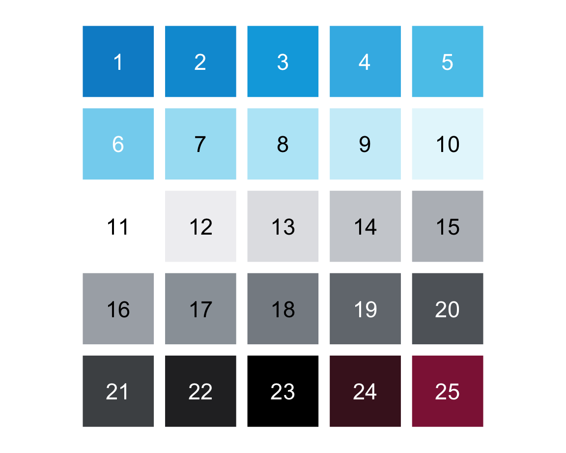
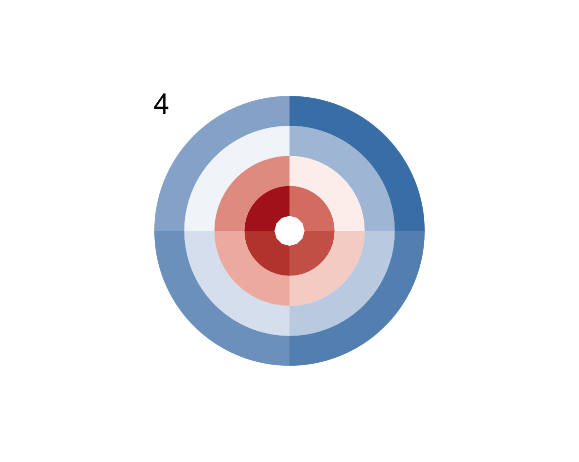
Hint: Check the documentation of plot_fun() (e.g., for color information).
1.8.3 Exercise 3
Dice sampling
In Section 1.6.4, we explored the coin() function of the ds4psy package and mimicked its functionality by the sample() function. In this exercise, we will explore the dice() and dice_2() functions of the same package.
Explore the
dice()function (of the ds4psy package) by first calling it a few times (with and without arguments). Then study its documentation (by calling?dice()).Explore the
dice_2()function (of the ds4psy package) by first calling it a few times (with and without arguments). Then study its documentation (by calling?dice_2()).
What are the differences between thedice()anddice_2()functions?Bonus task:29 Use the base R function
sample()to sample from the numbers1:6so thatsample()yields a fair dice in which all six numbers occur equally often, andsample()yields a biased dice in which the value6occurs twice as often as any other number.
Hint: The prob argument of sample() can be set to a vector of probability values
(i.e., as many values as length(x) that should sum up to a total value of 1).
1.8.4 Exercise 4
Cumulative savings
With only a little knowledge of R you can perform quite fancy financial arithmetic.
Assume that you have won an amount a of EUR 1000 and are considering to deposit this amount into a new bank account that offers an annual interest rate int of 0.1%.
How much would your account be worth after waiting for \(n = 2\) full years?
What would be the total value of your money after \(n = 2\) full years if the annual inflation rate
infis 2%?What would be the results to 1. and 2. if you waited for \(n = 10\) years?
Answer these questions by defining well-named objects and performing simple arithmetic computations on them.
Note:
Solving these tasks in R requires defining some numeric objects (e.g., a, int, and inf) and performing arithmetic computations with them (e.g., using +, *, ^, with appropriate parentheses).
Do not worry if you find these tasks difficult at this point — we will revisit them later.
In Exercise 6 of Chapter 12: Iteration, we will use loops and functions to solve such tasks in a more general fashion.
1.8.5 Exercise 5
Vector arithmetic
When introducing arithmetic functions above, we showed that they can be used with numeric scalars (i.e., numeric objects with a length of 1).
Demonstrate that arithmetic functions also work with two numeric vectors
xandy(of the same length).What happens when the vectors
xandyhave different lengths?
Hint: Define some numeric vectors and use them as arguments of various arithmetic functions. To better understand the behavior in 2., look up the term “recycling” in the context of R vectors.
1.8.6 Exercise 6
Cryptic arithmetic
Predict the result of the arithmetic expression x %/% y * y + x %% y.
Then test your prediction by assigning some positive number(s) to x and to y and evaluating the expression.
Finally, explain why the result occurs.
1.8.7 Exercise 7
Survey age
Assume the following definitions for a survey:
A person with an age from 1 to 17 years is classified as a minor;
a person with an age from 18 to 64 years is classified as an adult;
a person with an age from 65 to 99 years is classified as a senior.
Generate a vector with 100 random samples that specifies the age of 100 people (in years), but contains exactly 20 minors, 50 adults, and 30 seniors.
Now use some functions on your age vector to answer the following questions:
What is the average (mean), minimum, and maximum age in this sample?
How many people are younger than 25 years?
What is the average (mean) age of people older than 50 years?
How many people have a round age (i.e., an age that is divisible by 10)? What is their mean age?
1.8.8 Exercise 8
Exploring participant data
Explore the participant information of p_info (Woodworth, O’Brien-Malone, Diamond, & Schüz, 2018) by describing each of its variables:
How many individuals are contained in the dataset?
What percentage of them is female (i.e., has a
sexvalue of 1)?How many participants were in one of the 3 treatment groups (i.e., have an
interventionvalue of 1, 2, or 3)?What is the participants’ mean education level? What percentage has a university degree (i.e., an
educvalue of at least 4)?What is the age range (
mintomax) of participants? What is the average (mean and median) age?Describe the range of
incomelevels present in this sample of participants. What percentage of participants self-identifies as a below-average income (i.e., anincomevalue of 1)?Bonus task: The variables of
p_infoare stored as numeric variables, but some could also be factors.Which of the variables could or should be turned into factors?
It seems thatintervention,sex,educandincomecould/should be turned into factors.Recode some variables as factors (by consulting the codebook in Section 1.6.1).
Verify that the recoded factors correspond to the original variables.
Hint: The p_info data was defined and described above (in Section 1.6.1).
As it is also included as a tibble posPsy_p_info in the ds4psy package, it can be obtained by (re-)assigning:
p_info <- ds4psy::posPsy_p_infoThis concludes our first set of exercises on basic R concepts and commands.
References
Bonus in the sense of challenging, but rewarding when you solve it.↩︎