A.11 Solutions (11)

Here are the solutions of the basic exercises on creating functions of Chapter 11 (Section 11.6).
A.11.1 Exercise 1
Imagine someone proudly presents the following three functions to you.
Each of them takes a vector v as an input and tries to perform a simple task.
For each function:
- describe the task that the function is designed to perform,
- test whether it successfully performs this task,
- name any problem that you detect with the current function,
- fix the function so that it successfully performs its task.
# (1)  ------
first_element <- function(v) {

  output <- NA   # initialize
  output <- v[1] # set to 1st

}

# (2) ------
avg_mn_med <- function(v, na_rm = TRUE) {

  mn  <- mean(v)
  med <- median(v)
  avg <- (mn + med)/2

  return(avg)
}

# (3)  ------
mean_sd <- function(v, na_rm = TRUE) {

  mn  <- mean(v)
  sd  <- sd(v)

  both <- c(mn, sd)
  names(both) <- c("mean", "sd")

  return(mn)

}
Solution
Here are some statements suited to evaluate the functions (with various input arguments v):
# (1)  first_element aims to return the 1st element of a vector v.

# Check:
first_element(v = c(10, 11, 12))
first_element(v = c("A", "B", "C"))
first_element(v = c(NA, 11, 12))
first_element(v = NA)

# (2) avg_mn_med aims to compute 3 different metrics of centrality for v.

# Check:
avg_mn_med(v = c(1, 2, 3))
avg_mn_med(v = c(1, 2, 9))
avg_mn_med(v = c(1, 2, NA))
avg_mn_med(v = NA)
avg_mn_med(v = c("A", "B"))

# (3) mean_sd aims to compute the mean and standard deviation of v.

# Check:
mean_sd(v = c(1, 2, 3))
mean_sd(v = c(1, 2, 9))
mean_sd(v = c(1, 2, NA))
mean_sd(v = NA)
mean_sd(v = c("A", "B"))
Here are the same functions with some comments on shortcomings in their original definition and some quick fixes:
# (1)  ------
# Task: Return the 1st element of a vector v.
# Problem:  Nothing is returned.
# Solution: Add return(output).

first_element <- function(v) {

  output <- NA   # initialize
  output <- v[1] # set to 1st

  return(output)

}

# Check:
first_element(v = c(10, 11, 12))
#> [1] 10
first_element(v = c("A", "B", "C"))
#> [1] "A"
first_element(v = c(NA, 11, 12))
#> [1] NA
first_element(v = NA)
#> [1] NA

# (2) ------
# Task: Return the average of mean and median of v.
# Problem  1: na_rm is not used in function body.
# Solution 1: Add na_rm as value of the na.rm argument of base R functions.
# Problem  2: Function returns ERROR for non-numeric v.
# Solution 2: Use if statement to check for is.numeric(v).

avg_mn_med <- function(v, na_rm = TRUE) {

  if (!is.numeric(v)) {
    message("avg_mn_md: v requires numeric inputs.")
  } else {

    mn  <- mean(v, na.rm = na_rm)
    med <- median(v, na.rm = na_rm)
    avg <- (mn + med)/2

    return(avg)

  } # if (!is.numeric(v)) etc.
}

# Check:
avg_mn_med(v = c(1, 2, 3))
#> [1] 2
avg_mn_med(v = c(1, 2, 9))
#> [1] 3
avg_mn_med(v = c(1, 2, NA))
#> [1] 1.5
avg_mn_med(v = NA)
avg_mn_med(v = c("A", "B"))

# (3)  ------
# Task: Return the mean and sd of v.
# Problem  1: Only the mean is returned.
# Solution 1: return(both)
# Problem  2: na_rm is not used in function body.
# Solution 2: Add na_rm as value to na.rm of base functions.
# Problem  3: Function returns ERROR for non-numeric v.
# Solution 3: Use if statement to check for is.numeric(v).

mean_sd <- function(v, na_rm = TRUE) {

  if (all(is.na(v))) {return(v)}

  if (!is.numeric(v)) {
    message("mean_sd: v requires numeric inputs.")
  } else {

    mn  <- mean(v, na.rm = na_rm)
    sd  <- sd(v, na.rm = na_rm)

    both <- c(mn, sd)
    names(both) <- c("mean", "sd")

    return(both)

  } # if (!is.numeric(v)) etc.

}

# Check:
mean_sd(v = c(1, 2, 3))
#> mean   sd
#>    2    1
mean_sd(v = c(1, 2, 9))
#>     mean       sd
#> 4.000000 4.358899
mean_sd(v = c(1, 2, NA))
#>      mean        sd
#> 1.5000000 0.7071068
mean_sd(v = NA)
#> [1] NA
mean_sd(v = c("A", "B"))
A.11.2 Exercise 2
Conditional feeding
Let’s write a first function and then add some conditions to it.
- Write a function
feed_methat takes a character stringfoodas a required argument, and returns the sentence"I love to eat ___!". Test your function by runningfeed_me("apples"), etc.
Here’s a template with some blanks, to get you started:
feed_me <- function(___) {

  output <- paste0("I love to eat ", ___, "!")

  print(___)
}
Solution
A possible solution:
feed_me <- function(food) {

  output <- paste0("I love to eat ", food, "!")

  print(output)
  }

# Check:
feed_me("apples")
#> [1] "I love to eat apples!"
feed_me("books")
#> [1] "I love to eat books!"
feed_me("cake")
#> [1] "I love to eat cake!"
feed_me(NA)
#> [1] "I love to eat NA!"- Modify
feed_meso that it returns"Nothing to eat."whenfood = NA.
Solution
A possible solution:
feed_me <- function(food) {

  if (is.na(food)) {
    output <- "Nothing to eat."
  } else {
    output <- paste0("I love to eat ", food, "!")
  }

  print(output)
}

# Check:
feed_me(NA)
#> [1] "Nothing to eat."
feed_me("apples")
#> [1] "I love to eat apples!"
feed_me("books")
#> [1] "I love to eat books!"
Extend your function to a
feed_veganfunction that uses 2 additional arguments:typeshould be an optional character string, set to a default argument of"food". Iftypeis not"food", the function should return"___ is not edible.".veganshould be an optional Boolean value, which is set toFALSEby default. IfveganisTRUE, the function should return"I love to eat ___!". Otherwise, the function should return"I do not eat ___.".
Test each of your functions by evaluating appropriate function calls.
Solution
A possible solution:
feed_vegan <- function(food, type = "food", vegan = FALSE) {

  if (is.na(food)) {

    output <- "Nothing to eat."

  } else {  # food is not NA:

    if (type != "food") {
      output <- paste0(food, " is not edible.")
    } else {  # type == "food":

      if (vegan) {
        output <- paste0("I love to eat ", food, "!")
      } else {  # vegan
        output <- paste0("I do not eat ", food, ".")
      }
    }
  }

  print(output)
}

# Check:
feed_vegan(NA)
#> [1] "Nothing to eat."
feed_vegan("veggies", vegan = TRUE)
#> [1] "I love to eat veggies!"
feed_vegan("R4DS", type = "book")
#> [1] "R4DS is not edible."
feed_vegan("meat", vegan = FALSE)
#> [1] "I do not eat meat."
# but:
feed_vegan("spagetti", type = "pasta")  # due to type != "food"
#> [1] "spagetti is not edible."
feed_vegan("veggies")  # due to default: vegan = FALSE
#> [1] "I do not eat veggies."
A.11.3 Exercise 3
Number recognition
This exercise analyzes and corrects someone else’s function.
- Explain what the following function
describe(not to be confused withdescribeabove) intends to do and why it fails in doing it.
describe <- function(x) {

  if (x %% 2 == 0)  {print("x is an even number.")}
  else if (x %% 2 == 1) {print("x is an odd number.")}
  else if (x < 1)   {print("x is too small.")}
  else if (x > 20)  {print("x is too big.")}
  else if (x == 13) {print("x is a lucky number.")}
  else if (x == pi) {print("Let's make a pie!")}
  else {print("x is beyond description.")}

}
Solution
The function describe seems to want to categorize a number x into one of various cases:
- numbers that are too small numbers vs. too big
- odd vs. even numbers
- 13 as a lucky number
pito make a pie
- numbers that cannot be described
However, it currently fails (and only distinguishes between even and odd numbers), because of the order of its if statements. Currently, the quite general tests at the beginning are TRUE for most cases, so that more specific later cases are never reached.
- Repair the
describefunction to yield the following results:
# Desired results:
describe(0)
#> [1] "x is too small."
describe(1)
#> [1] "x is an odd number."
describe(13)
#> [1] "x is a lucky number."
describe(20)
#> [1] "x is an even number."
describe(21)
#> [1] "x is too big."
describe(pi)
#> [1] "Let's make a pie!"
Solution
To repair the function, we need to re-arrange the if statements (putting some more specific statements before more general ones):
# Correction:
describe <- function(x) {

  if (x < 1)            {print("x is too small.")}
  else if (x > 20)      {print("x is too big.")}
  else if (x == 13)     {print("x is a lucky number.")}
  else if (x %% 2 == 0) {print("x is an even number.")}
  else if (x %% 2 == 1) {print("x is an odd number.")}
  else if (x == pi)     {print("Let's make a pie!")}
  else                  {print("x is beyond description.")}

}

# Check:
describe(0)
#> [1] "x is too small."
describe(1)
#> [1] "x is an odd number."
describe(13)
#> [1] "x is a lucky number."
describe(20)
#> [1] "x is an even number."
describe(21)
#> [1] "x is too big."
describe(pi)
#> [1] "Let's make a pie!"- What are the results of
describe(NA)anddescribe("one")? Correct the function to yield appropriate results in both cases.
Solution
# Check:
# describe(NA)   # yields an ERROR
describe("one")  # yields "x is too big."
#> [1] "x is too big."
"one" > 20       # is TRUE!
#> [1] TRUE

# Correction:
describe <- function(x) {

  # stopifnot(!is.na(x))  # would yield an error if is.na(x)

  if (is.na(x))         {print("x is NA.")}
  else if (is.character(x)) {print("x is a word.")}

  else if (x < 1)       {print("x is too small.")}
  else if (x > 20)      {print("x is too big.")}
  else if (x == 13)     {print("x is a lucky number.")}
  else if (x %% 2 == 0) {print("x is an even number.")}
  else if (x %% 2 == 1) {print("x is an odd number.")}
  else if (x == pi)     {print("Let's make a pie!")}
  else                  {print("x is beyond description.")}

}

# Check:
describe(NA)     # yields "x is NA."
#> [1] "x is NA."
describe("one")  # yields "x is a word."
#> [1] "x is a word."- For what kind of
xwilldescribeprint"x is beyond description."?
Solution
The describe() function prints "x is beyond description." for values of 1 < x < 20 that are not integers and not pi:
# For 1 < x < 20 that are not integers:
describe(3/2)
#> [1] "x is beyond description."
describe(sqrt(2))
#> [1] "x is beyond description."
describe(pi + .001)
#> [1] "x is beyond description."
# but:
describe(pi)
#> [1] "Let's make a pie!"
A.11.4 Exercise 4
Double standards?
Smart Alex is a student in this course, whereas Smart Alexa has graduated and now works as a software developer for a company.
Both get the assignment to define a fac() function that computes the factorial of some number n and submit the following solution:
fac <- function(n){

  factorial(n)

}
Surprisingly, the consequences differ: Whereas Smart Alex gets a bad grade, Smart Alexa gets promoted. Explain.
Solution
Their solution for fac(n) works, of course, but only by passing n to the in-built base R function factorial().
As a student of this course, Smart Alex was asked for solving the problem in a principled way (e.g., by simplifying it and using recursion). By contrast, Smart Alexa works in a practical context and does the right thing by simply using an optimized and proven solution to the problem, rather than wasting time and effort by creating another (and often inferior) solution.
Another way of expressing this emphasizes that the context is a part of someone’s task: While both individuals have provided the same solution, they were actually facing different tasks. Given the educational context of Alex’s problem, Alexa’s excellent solution did not qualify as a “solution.”
A.11.5 Exercise 5
Randomizers revisited
In Chapter 1, we explored the ds4psy functions coin(), dice(), and dice_2(), and used the base R function sample() to mimic their behavior (see Section 1.6.4 and Exercise 3 in Section 1.8.3).
Now we can create these functions.
- Study the
dice()function of ds4psy and write a functionmy_dice()that accepts one argumentNand always returnsNrandom numbers from 1 to 6 (as a number).
Hint: Drawing random numbers from a uniform distribution could be achieved by stats::runif(), but beware of distortions when rounding its results. An easier solution uses the base::sample() function in its definition.
Solution
We create two versions:
- Use only one argument
N, but specifyeventsinside the function body:
# (1) Solution: Wrapping the sample() function
my_dice <- function(N = 1){

  events <- 1:6

  out <- base::sample(x = events, size = N, replace = TRUE)

  return(out)

}

# Check:
my_dice()
#> [1] 6
my_dice(5)
#> [1] 3 4 2 4 2
table(my_dice(6000))
#>
#>    1    2    3    4    5    6
#> 1038 972 1002 978 1005 1005- Use two arguments
Nandeventsand pass them to eithersample()ordice():
# (2) Just wrapping the existing dice() function:
my_dice_2 <- function(N = 1, events = 1:6){

  ## (a) Use sample():
  # base::sample(x = events, size = N, replace = TRUE)

  # (b) Use dice() (which also uses sample()):
  ds4psy::dice(n = N, events = events)

}

# Check:
my_dice_2()
#> [1] 4
my_dice_2(5)
#> [1] 1 5 2 6 6
table(my_dice_2(6000))
#>
#>    1    2    3    4    5    6
#>  989 1019 1008 1009  977  998
Note: Both solutions shown here write a new function by primarily passing arguments to an existing function. In such cases, we should ask ourselves whether the new function is really needed. If we decide that it is and we use this method, we should be confident that (a) we understand the function to which we are passing our arguments and (b) that this function is working properly. For this reason, it is generally safer to use base R functions in our functions than those of less established packages. (In addition, using functions from other packages makes your code dependent on those packages. Dependencies become an important consideration when writing your own packages.)
- Use (parts of) your new
my_dice()function to write amy_coin()function that mimicks the behavior of the ds4psycoin()function.
Hint: The sampling part of the function remains the same — only the events to sample from change.
Solution
We create two versions:
- If our
my_dice()function has no argument for specifyingevents:
my_coin <- function(N = 1){

  events <- c("H", "T")

  out <- base::sample(x = events, size = N, replace = TRUE)

  return(out)

}

# Check:
my_coin()
#> [1] "H"
my_coin(5)
#> [1] "H" "H" "T" "T" "T"
table(my_coin(2000))
#>
#>    H    T
#> 1041 959- If our
my_dice()function has an argument for specifyingevents:
my_coin_2 <- function(N = 1, events = c("H", "T")){

  my_dice_2(N = N, events = events)

}

# Check:
my_coin_2()
#> [1] "H"
my_coin_2(5)
#> [1] "T" "H" "H" "H" "H"

# Notes:
# my_dice_2() can mimic the coin() function:
my_dice_2(10, events = c("H", "T"))  #
#>  [1] "T" "H" "H" "H" "H" "T" "H" "H" "H" "H"
table(my_dice_2(1000, events = c("H", "T")))
#>
#>   H   T
#> 488 512

# We can use functions for imitating other functions:
my_coin_2(6, events = LETTERS[1:3])
#> [1] "C" "C" "B" "C" "B" "B"
Note:
Our two versions my_coin() and my_coin_2() differ in their direct dependencies (on either base::sample() or our own my_dice_2() function) and their generality: Whereas the set of possible events is fixed in my_coin() (by being defined inside the function body) it is left up to the user in my_coin_2() (by being an argument of the function). Thus, writing functions always involves decisions regarding their dependencies, flexibility, and scope.
- Bonus task: We have seen (in Exercise 3, Section 1.8.3) that the
dice_2()function of ds4psy yields non-random results. Write a similarmy_special_dice()function that accepts two arguments:
Nis the number of dice to throw. Each dice should always yield a number from 1 to 6 and your function should return theNnumbers of the set of dice.The 2nd argument
special_numberlets you specify a number (from 1 to 6) that will occur twice as often as the other numbers in exactly one of the dice.To make this scam less obvious, your function should return the results of the
Ndice in a random order.
Hint: We can rely on the dice() function to imitate all dice. For the one “special” dice, we need to change the events to sample from so that the special_number occurs twice as often as the other numbers. Randomizing the order of outputs can be achieved by the sample() function (by drawing N dice from the set of all dice without replacement).
Solution
# Re-examining dice_2():
table(dice_2(n = 30000, sides = 1:3))
#>
#>     1     2     3
#>  9734  9523 10743

# New function:
my_special_dice <- function(N = 1, special_number = NA){

  out <- NA
  special <- NA
  others <- NULL

  events <- 1:6

  # 1 special dice:
  if (is.na(special_number)){

    special <- ds4psy::dice(n = 1, events = events)

  } else {

    # Sample so that special_number occurs twice as often as any other number:
    special_sample <- rep(special_number, 2)  # consider special_number TWICE
    other_sample <- events[-special_number]   # events WITHOUT special_number
    total_sample <- c(special_sample, other_sample)

    special <- sample(x = total_sample, size = 1)
  }

  # All other dice:
  if (N > 1){
    others <- ds4psy::dice(n = (N - 1), events = events)
  }

  # Combine results:
  out <- c(special, others)

  # Randomize the order of out:
  out <- sample(x = out, size = length(out), replace = FALSE)

  # Return:
  return(out)

}

# Check:
my_special_dice()
#> [1] 3
my_special_dice(N = 10)
#>  [1] 3 3 2 3 1 4 4 6 6 1
my_special_dice(N = 10, special_number = 4)
#> [1] 2 5 1 3 3 5 1 1 4 2- Bonus task:
- How could you check whether your
my_special_dice()function works as intended?
Hint: Don’t solve it here — just describe what you would need to check your function.
Solution
As my_special_dice() lacks an argument to throw the set of dice repeatedly, we would need to call it many times to detect which of the N dice is non-random and whether it behaves as intended (i.e., special_number occurring twice as often as any other number). This can be solved with a loop, as we will see in the next Chapter 12 on Iteration.
A.11.6 Exercise 6
Tibble charts
This exercise writes a function to extract rows from tabular inputs based on the top values of some variable.
- Write a
top_3function that takes a tibbledataand a the column numbercol_nrof a numeric variable as its 2 inputs and returns the top-3 rows of the tibble after it has been sorted (in descending order) by the specified column number.
Use the data of sw <- dplyr::starwars to illustrate your function.
Hint: To write this function, first solve its task for a specific case (e.g., for col_nr = 2).
When using the dplyr commands of the tidyverse, a problem you will encounter is that a tibble’s variables are typically referenced by their unquoted names, rather than by their number (or column index). Here are 2 ways to solve this problem:
To obtain the unquoted name
some_nameof a given character string"some_name", you can call!!sym("some_name").Rather than aiming for a tidyverse solution, you could solve the problem with base R commands. In this case, look up and use the command
orderto re-arrange the rows of a tibble or data frame.
Solution
- A possible tidyverse solution:
# Data:
sw <- dplyr::starwars

# (a) specific solution:
# dplyr-pipe solution uses unquoted variable name:
sw %>% arrange(desc(height)) %>% slice(1:3)
#> # A tibble: 3 × 14
#>   name     height  mass hair_color skin_color eye_color birth_year sex   gender
#>   <chr>     <int> <dbl> <chr>      <chr>      <chr>          <dbl> <chr> <chr>
#> 1 Yarael …    264    NA none       white      yellow            NA male  mascul…
#> 2 Tarfful     234   136 brown      brown      blue              NA male  mascul…
#> 3 Lama Su     229    88 none       grey       black             NA male  mascul…
#> # … with 5 more variables: homeworld <chr>, species <chr>, films <list>,
#> #   vehicles <list>, starships <list>

# (b) Same pipe with a quoted variable name:
sw %>% arrange(desc(!!sym("height"))) %>% slice(1:3)
#> # A tibble: 3 × 14
#>   name     height  mass hair_color skin_color eye_color birth_year sex   gender
#>   <chr>     <int> <dbl> <chr>      <chr>      <chr>          <dbl> <chr> <chr>
#> 1 Yarael …    264    NA none       white      yellow            NA male  mascul…
#> 2 Tarfful     234   136 brown      brown      blue              NA male  mascul…
#> 3 Lama Su     229    88 none       grey       black             NA male  mascul…
#> # … with 5 more variables: homeworld <chr>, species <chr>, films <list>,
#> #   vehicles <list>, starships <list>

# (c) Translation into a function:
top_3 <- function(data, col_nr){

  col_name <- names(data)[col_nr]

  result <- data %>%
    arrange(desc(!!sym(col_name))) %>%
    slice(1:3)

  return(result)

}
Checking the top_3() function:
# Check:
top_3(sw, 2)  # top_3 height values
#> # A tibble: 3 × 14
#>   name     height  mass hair_color skin_color eye_color birth_year sex   gender
#>   <chr>     <int> <dbl> <chr>      <chr>      <chr>          <dbl> <chr> <chr>
#> 1 Yarael …    264    NA none       white      yellow            NA male  mascul…
#> 2 Tarfful     234   136 brown      brown      blue              NA male  mascul…
#> 3 Lama Su     229    88 none       grey       black             NA male  mascul…
#> # … with 5 more variables: homeworld <chr>, species <chr>, films <list>,
#> #   vehicles <list>, starships <list>
top_3(sw, 3)  # top_3 mass values
#> # A tibble: 3 × 14
#>   name    height  mass hair_color skin_color  eye_color  birth_year sex   gender
#>   <chr>    <int> <dbl> <chr>      <chr>       <chr>           <dbl> <chr> <chr>
#> 1 Jabba …    175  1358 <NA>       green-tan,… orange            600 herm… mascu…
#> 2 Grievo…    216   159 none       brown, whi… green, ye…         NA male  mascu…
#> 3 IG-88      200   140 none       metal       red                15 none  mascu…
#> # … with 5 more variables: homeworld <chr>, species <chr>, films <list>,
#> #   vehicles <list>, starships <list>
top_3(sw, 7)  # top_3 birth_year values
#> # A tibble: 3 × 14
#>   name    height  mass hair_color skin_color  eye_color birth_year sex    gender
#>   <chr>    <int> <dbl> <chr>      <chr>       <chr>          <dbl> <chr>  <chr>
#> 1 Yoda        66    17 white      green       brown            896 male   mascu…
#> 2 Jabba …    175  1358 <NA>       green-tan,… orange           600 herma… mascu…
#> 3 Chewba…    228   112 brown      unknown     blue             200 male   mascu…
#> # … with 5 more variables: homeworld <chr>, species <chr>, films <list>,
#> #   vehicles <list>, starships <list>
# But:
top_3(sw, 1)  # character variables are ordered in reverse of alphabetical order
#> # A tibble: 3 × 14
#>   name    height  mass hair_color skin_color   eye_color birth_year sex   gender
#>   <chr>    <int> <dbl> <chr>      <chr>        <chr>          <dbl> <chr> <chr>
#> 1 Zam We…    168    55 blonde     fair, green… yellow            NA fema… femin…
#> 2 Yoda        66    17 white      green        brown            896 male  mascu…
#> 3 Yarael…    264    NA none       white        yellow            NA male  mascu…
#> # … with 5 more variables: homeworld <chr>, species <chr>, films <list>,
#> # vehicles <list>, starships <list>- A solution using only base R functions (here:
order()):
# Data:
sw <- dplyr::starwars

# (a) specific solution for sorting data:
# using order() function and a variable name:
sw[order(-sw$height), ]
#> # A tibble: 87 × 14
#>    name    height  mass hair_color skin_color  eye_color birth_year sex   gender
#>    <chr>    <int> <dbl> <chr>      <chr>       <chr>          <dbl> <chr> <chr>
#>  1 Yarael…    264    NA none       white       yellow          NA   male  mascu…
#>  2 Tarfful    234   136 brown      brown       blue            NA   male  mascu…
#>  3 Lama Su    229    88 none       grey        black           NA   male  mascu…
#>  4 Chewba…    228   112 brown      unknown     blue           200   male  mascu…
#>  5 Roos T…    224    82 none       grey        orange          NA   male  mascu…
#>  6 Grievo…    216   159 none       brown, whi… green, y…       NA   male  mascu…
#>  7 Taun We    213    NA none       grey        black           NA   fema… femin…
#>  8 Rugor …    206    NA none       green       orange          NA   male  mascu…
#>  9 Tion M…    206    80 none       grey        black           NA   male  mascu…
#> 10 Darth …    202   136 none       white       yellow          41.9 male  mascu…
#> # … with 77 more rows, and 5 more variables: homeworld <chr>, species <chr>,
#> #   films <list>, vehicles <list>, starships <list>

# Note:
sw$height # is a vector (of height values)
#>  [1] 172 167  96 202 150 178 165  97 183 182 188 180 228 180 173 175 170 180  66
#> [20] 170 183 200 190 177 175 180 150  NA  88 160 193 191 170 196 224 206 183 137
#> [39] 112 183 163 175 180 178  94 122 163 188 198 196 171 184 188 264 188 196 185
#> [58] 157 183 183 170 166 165 193 191 183 168 198 229 213 167  79  96 193 191
#>  [ reached getOption("max.print") -- omitted 12 entries ]
sw[ , 2]  # is the same vector (as column of sw)
#> # A tibble: 87 × 1
#>    height
#>     <int>
#>  1    172
#>  2    167
#>  3     96
#>  4    202
#>  5    150
#>  6    178
#>  7    165
#>  8     97
#>  9    183
#> 10    182
#> # … with 77 more rows

# (b) specific solution for sorting data:
# using order() function and the variable's column number:
sw[order(-sw[ , 2]), ]
#> # A tibble: 87 × 14
#>    name    height  mass hair_color skin_color  eye_color birth_year sex   gender
#>    <chr>    <int> <dbl> <chr>      <chr>       <chr>          <dbl> <chr> <chr>
#>  1 Yarael…    264    NA none       white       yellow          NA   male  mascu…
#>  2 Tarfful    234   136 brown      brown       blue            NA   male  mascu…
#>  3 Lama Su    229    88 none       grey        black           NA   male  mascu…
#>  4 Chewba…    228   112 brown      unknown     blue           200   male  mascu…
#>  5 Roos T…    224    82 none       grey        orange          NA   male  mascu…
#>  6 Grievo…    216   159 none       brown, whi… green, y…       NA   male  mascu…
#>  7 Taun We    213    NA none       grey        black           NA   fema… femin…
#>  8 Rugor …    206    NA none       green       orange          NA   male  mascu…
#>  9 Tion M…    206    80 none       grey        black           NA   male  mascu…
#> 10 Darth …    202   136 none       white       yellow          41.9 male  mascu…
#> # … with 77 more rows, and 5 more variables: homeworld <chr>, species <chr>,
#> #   films <list>, vehicles <list>, starships <list>

# (c) Translation into a function:
top_3_base <- function(data, col_nr){

  sorted_data <- data[order(-data[ , col_nr]), ]

  result <- sorted_data[1:3, ]  # top 3 rows

  return(result)

}
Checking the top_3_base() function:
# Check:
top_3_base(sw, 2)  # top_3 height values
#> # A tibble: 3 × 14
#>   name     height  mass hair_color skin_color eye_color birth_year sex   gender
#>   <chr>     <int> <dbl> <chr>      <chr>      <chr>          <dbl> <chr> <chr>
#> 1 Yarael …    264    NA none       white      yellow            NA male  mascul…
#> 2 Tarfful     234   136 brown      brown      blue              NA male  mascul…
#> 3 Lama Su     229    88 none       grey       black             NA male  mascul…
#> # … with 5 more variables: homeworld <chr>, species <chr>, films <list>,
#> #   vehicles <list>, starships <list>
top_3_base(sw, 3)  # top_3 mass values
#> # A tibble: 3 × 14
#>   name    height  mass hair_color skin_color  eye_color  birth_year sex   gender
#>   <chr>    <int> <dbl> <chr>      <chr>       <chr>           <dbl> <chr> <chr>
#> 1 Jabba …    175  1358 <NA>       green-tan,… orange            600 herm… mascu…
#> 2 Grievo…    216   159 none       brown, whi… green, ye…         NA male  mascu…
#> 3 IG-88      200   140 none       metal       red                15 none  mascu…
#> # … with 5 more variables: homeworld <chr>, species <chr>, films <list>,
#> #   vehicles <list>, starships <list>
top_3_base(sw, 7)  # top_3 birth_year values
#> # A tibble: 3 × 14
#>   name    height  mass hair_color skin_color  eye_color birth_year sex    gender
#>   <chr>    <int> <dbl> <chr>      <chr>       <chr>          <dbl> <chr>  <chr>
#> 1 Yoda        66    17 white      green       brown            896 male   mascu…
#> 2 Jabba …    175  1358 <NA>       green-tan,… orange           600 herma… mascu…
#> 3 Chewba…    228   112 brown      unknown     blue             200 male   mascu…
#> # … with 5 more variables: homeworld <chr>, species <chr>, films <list>,
#> #   vehicles <list>, starships <list>
# But:
# top_3_base(sw, 1)  # would yield an error, as order does not allow "-" for character variables.
What happens in your
top_3function whencol_nrrefers to a character variable (e.g.,dplyr::starwars[ , 1])? Adjust the function so that its result varies by the type of the variable designated by thecol_nrargument:- if the corresponding variable is a character variable, sort the data in ascending order (alphabetically);
- if the corresponding variable is a numeric variable, sort the data in descending order (from high to low).
Solution
- Adjusted tidyverse solution:
# What happens?
top_3(sw, 1)  # character variables are ordered in reverse of alphabetical order
#> # A tibble: 3 × 14
#>   name    height  mass hair_color skin_color   eye_color birth_year sex   gender
#>   <chr>    <int> <dbl> <chr>      <chr>        <chr>          <dbl> <chr> <chr>
#> 1 Zam We…    168    55 blonde     fair, green… yellow            NA fema… femin…
#> 2 Yoda        66    17 white      green        brown            896 male  mascu…
#> 3 Yarael…    264    NA none       white        yellow            NA male  mascu…
#> # … with 5 more variables: homeworld <chr>, species <chr>, films <list>,
#> #   vehicles <list>, starships <list>

# Preparation: How can we determine the variable type?
# character variable:
sw$name   # a vector name in sw
#>  [1] "Luke Skywalker"        "C-3PO"                 "R2-D2"
#>  [4] "Darth Vader"           "Leia Organa"           "Owen Lars"
#>  [7] "Beru Whitesun lars"    "R5-D4"                 "Biggs Darklighter"
#> [10] "Obi-Wan Kenobi"        "Anakin Skywalker"      "Wilhuff Tarkin"
#> [13] "Chewbacca"             "Han Solo"              "Greedo"
#> [16] "Jabba Desilijic Tiure" "Wedge Antilles"        "Jek Tono Porkins"
#> [19] "Yoda"                  "Palpatine"             "Boba Fett"
#> [22] "IG-88"                 "Bossk"                 "Lando Calrissian"
#> [25] "Lobot"                 "Ackbar"                "Mon Mothma"
#> [28] "Arvel Crynyd"          "Wicket Systri Warrick" "Nien Nunb"
#> [31] "Qui-Gon Jinn"          "Nute Gunray"           "Finis Valorum"
#> [34] "Jar Jar Binks"         "Roos Tarpals"          "Rugor Nass"
#> [37] "Ric Olié"              "Watto"                 "Sebulba"
#> [40] "Quarsh Panaka"         "Shmi Skywalker"        "Darth Maul"
#> [43] "Bib Fortuna"           "Ayla Secura"           "Dud Bolt"
#> [46] "Gasgano"               "Ben Quadinaros"        "Mace Windu"
#> [49] "Ki-Adi-Mundi"          "Kit Fisto"             "Eeth Koth"
#> [52] "Adi Gallia"            "Saesee Tiin"           "Yarael Poof"
#> [55] "Plo Koon"              "Mas Amedda"            "Gregar Typho"
#> [58] "Cordé"                 "Cliegg Lars"           "Poggle the Lesser"
#> [61] "Luminara Unduli"       "Barriss Offee"         "Dormé"
#> [64] "Dooku"                 "Bail Prestor Organa"   "Jango Fett"
#> [67] "Zam Wesell"            "Dexter Jettster"       "Lama Su"
#> [70] "Taun We"               "Jocasta Nu"            "Ratts Tyerell"
#> [73] "R4-P17"                "Wat Tambor"            "San Hill"
#>  [ reached getOption("max.print") -- omitted 12 entries ]
sw[ , 1]  # 1st column of sw
#> # A tibble: 87 × 1
#>    name
#>    <chr>
#>  1 Luke Skywalker
#>  2 C-3PO
#>  3 R2-D2
#>  4 Darth Vader
#>  5 Leia Organa
#>  6 Owen Lars
#>  7 Beru Whitesun lars
#>  8 R5-D4
#>  9 Biggs Darklighter
#> 10 Obi-Wan Kenobi
#> # … with 77 more rows

typeof(sw$name)  # character
#> [1] "character"
typeof(sw[ , 1]) # list!
#> [1] "list"
typeof(unlist(sw[ , 1])) # character !!
#> [1] "character"
typeof(sw[[1]])  # character
#> [1] "character"

# numeric variable:
sw$height  # a vector height in sw
#>  [1] 172 167  96 202 150 178 165  97 183 182 188 180 228 180 173 175 170 180  66
#> [20] 170 183 200 190 177 175 180 150  NA  88 160 193 191 170 196 224 206 183 137
#> [39] 112 183 163 175 180 178  94 122 163 188 198 196 171 184 188 264 188 196 185
#> [58] 157 183 183 170 166 165 193 191 183 168 198 229 213 167  79  96 193 191
#>  [ reached getOption("max.print") -- omitted 12 entries ]
sw[ , 2]   # 2nd column of sw
#> # A tibble: 87 × 1
#>    height
#>     <int>
#>  1    172
#>  2    167
#>  3     96
#>  4    202
#>  5    150
#>  6    178
#>  7    165
#>  8     97
#>  9    183
#> 10    182
#> # … with 77 more rows
sw[[2]]    # as a vector
#>  [1] 172 167  96 202 150 178 165  97 183 182 188 180 228 180 173 175 170 180  66
#> [20] 170 183 200 190 177 175 180 150  NA  88 160 193 191 170 196 224 206 183 137
#> [39] 112 183 163 175 180 178  94 122 163 188 198 196 171 184 188 264 188 196 185
#> [58] 157 183 183 170 166 165 193 191 183 168 198 229 213 167  79  96 193 191
#>  [ reached getOption("max.print") -- omitted 12 entries ]

typeof(sw$height)  # integer
#> [1] "integer"
typeof(sw[ , 2])   # list!
#> [1] "list"
typeof(unlist(sw[ , 2])) # integer
#> [1] "integer"
typeof(sw[[2]])    # integer
#> [1] "integer"

# Adjusting function from above:
top_3 <- function(data, col_nr){

  col_name <- names(data)[col_nr]
  col_type <- typeof(unlist(data[ , col_nr]))

  if (col_type == "character") {

    result <- data %>%
      arrange(!!sym(col_name)) %>%  # do NOT use desc()
      slice(1:3)

  } else {  # col_type != "character"

    result <- data %>%
      arrange(desc(!!sym(col_name))) %>%
      slice(1:3)

  }

  return(result)

}
Checking this top_3() function:
# Check:
top_3(sw, 2)  # top_3 height values
#> # A tibble: 3 × 14
#>   name     height  mass hair_color skin_color eye_color birth_year sex   gender
#>   <chr>     <int> <dbl> <chr>      <chr>      <chr>          <dbl> <chr> <chr>
#> 1 Yarael …    264    NA none       white      yellow            NA male  mascul…
#> 2 Tarfful     234   136 brown      brown      blue              NA male  mascul…
#> 3 Lama Su     229    88 none       grey       black             NA male  mascul…
#> # … with 5 more variables: homeworld <chr>, species <chr>, films <list>,
#> #   vehicles <list>, starships <list>
top_3(sw, 3)  # top_3 mass values
#> # A tibble: 3 × 14
#>   name    height  mass hair_color skin_color  eye_color  birth_year sex   gender
#>   <chr>    <int> <dbl> <chr>      <chr>       <chr>           <dbl> <chr> <chr>
#> 1 Jabba …    175  1358 <NA>       green-tan,… orange            600 herm… mascu…
#> 2 Grievo…    216   159 none       brown, whi… green, ye…         NA male  mascu…
#> 3 IG-88      200   140 none       metal       red                15 none  mascu…
#> # … with 5 more variables: homeworld <chr>, species <chr>, films <list>,
#> #   vehicles <list>, starships <list>
top_3(sw, 7)  # top_3 birth_year values
#> # A tibble: 3 × 14
#>   name    height  mass hair_color skin_color  eye_color birth_year sex    gender
#>   <chr>    <int> <dbl> <chr>      <chr>       <chr>          <dbl> <chr>  <chr>
#> 1 Yoda        66    17 white      green       brown            896 male   mascu…
#> 2 Jabba …    175  1358 <NA>       green-tan,… orange           600 herma… mascu…
#> 3 Chewba…    228   112 brown      unknown     blue             200 male   mascu…
#> # … with 5 more variables: homeworld <chr>, species <chr>, films <list>,
#> #   vehicles <list>, starships <list>
# AND now:
top_3(sw, 1)  # name in alphabetical order
#> # A tibble: 3 × 14
#>   name     height  mass hair_color skin_color  eye_color birth_year sex   gender
#>   <chr>     <int> <dbl> <chr>      <chr>       <chr>          <dbl> <chr> <chr>
#> 1 Ackbar      180    83 none       brown mott… orange          41   male  mascu…
#> 2 Adi Gal…    184    50 none       dark        blue            NA   fema… femin…
#> 3 Anakin …    188    84 blond      fair        blue            41.9 male  mascu…
#> # … with 5 more variables: homeworld <chr>, species <chr>, films <list>,
#> #   vehicles <list>, starships <list>
top_3(sw, 9)  # homeworld in alphabetical order
#> # A tibble: 3 × 14
#>   name      height  mass hair_color skin_color eye_color birth_year sex   gender
#>   <chr>      <int> <dbl> <chr>      <chr>      <chr>          <dbl> <chr> <chr>
#> 1 Leia Org…    150    49 brown      light      brown             19 fema… femin…
#> 2 Beru Whi…    165    75 brown      light      blue              47 fema… femin…
#> 3 Mon Moth…    150    NA auburn     fair       blue              48 fema… femin…
#> # … with 5 more variables: homeworld <chr>, species <chr>, films <list>,
#> # vehicles <list>, starships <list>- Adjusted base R solution:
# What happens?
# top_3_base(sw, 1)  # would yield an error, as order does not allow "-" for character variables.

# (a) specific solution for sorting data:
# using order() function and a variable name:
sw[order(-sw$height), ]
#> # A tibble: 87 × 14
#>    name    height  mass hair_color skin_color  eye_color birth_year sex   gender
#>    <chr>    <int> <dbl> <chr>      <chr>       <chr>          <dbl> <chr> <chr>
#>  1 Yarael…    264    NA none       white       yellow          NA   male  mascu…
#>  2 Tarfful    234   136 brown      brown       blue            NA   male  mascu…
#>  3 Lama Su    229    88 none       grey        black           NA   male  mascu…
#>  4 Chewba…    228   112 brown      unknown     blue           200   male  mascu…
#>  5 Roos T…    224    82 none       grey        orange          NA   male  mascu…
#>  6 Grievo…    216   159 none       brown, whi… green, y…       NA   male  mascu…
#>  7 Taun We    213    NA none       grey        black           NA   fema… femin…
#>  8 Rugor …    206    NA none       green       orange          NA   male  mascu…
#>  9 Tion M…    206    80 none       grey        black           NA   male  mascu…
#> 10 Darth …    202   136 none       white       yellow          41.9 male  mascu…
#> # … with 77 more rows, and 5 more variables: homeworld <chr>, species <chr>,
#> #   films <list>, vehicles <list>, starships <list>

# as above:
typeof(unlist(sw[ , 1]))  # "character"
#> [1] "character"
typeof(unlist(sw[ , 2]))  # "integer"
#> [1] "integer"
typeof(unlist(sw[ , 3]))  # "double"
#> [1] "double"
typeof(sw[[3]])           # "double"
#> [1] "double"

sw[order(sw$name), ] # works
#> # A tibble: 87 × 14
#>    name    height  mass hair_color skin_color  eye_color birth_year sex   gender
#>    <chr>    <int> <dbl> <chr>      <chr>       <chr>          <dbl> <chr> <chr>
#>  1 Ackbar     180    83 none       brown mott… orange          41   male  mascu…
#>  2 Adi Ga…    184    50 none       dark        blue            NA   fema… femin…
#>  3 Anakin…    188    84 blond      fair        blue            41.9 male  mascu…
#>  4 Arvel …     NA    NA brown      fair        brown           NA   male  mascu…
#>  5 Ayla S…    178    55 none       blue        hazel           48   fema… femin…
#>  6 Bail P…    191    NA black      tan         brown           67   male  mascu…
#>  7 Barris…    166    50 black      yellow      blue            40   fema… femin…
#>  8 BB8         NA    NA none       none        black           NA   none  mascu…
#>  9 Ben Qu…    163    65 none       grey, gree… orange          NA   male  mascu…
#> 10 Beru W…    165    75 brown      light       blue            47   fema… femin…
#> # … with 77 more rows, and 5 more variables: homeworld <chr>, species <chr>,
#> #   films <list>, vehicles <list>, starships <list>
sw$name # is a vector
#>  [1] "Luke Skywalker"        "C-3PO"                 "R2-D2"
#>  [4] "Darth Vader"           "Leia Organa"           "Owen Lars"
#>  [7] "Beru Whitesun lars"    "R5-D4"                 "Biggs Darklighter"
#> [10] "Obi-Wan Kenobi"        "Anakin Skywalker"      "Wilhuff Tarkin"
#> [13] "Chewbacca"             "Han Solo"              "Greedo"
#> [16] "Jabba Desilijic Tiure" "Wedge Antilles"        "Jek Tono Porkins"
#> [19] "Yoda"                  "Palpatine"             "Boba Fett"
#> [22] "IG-88"                 "Bossk"                 "Lando Calrissian"
#> [25] "Lobot"                 "Ackbar"                "Mon Mothma"
#> [28] "Arvel Crynyd"          "Wicket Systri Warrick" "Nien Nunb"
#> [31] "Qui-Gon Jinn"          "Nute Gunray"           "Finis Valorum"
#> [34] "Jar Jar Binks"         "Roos Tarpals"          "Rugor Nass"
#> [37] "Ric Olié"              "Watto"                 "Sebulba"
#> [40] "Quarsh Panaka"         "Shmi Skywalker"        "Darth Maul"
#> [43] "Bib Fortuna"           "Ayla Secura"           "Dud Bolt"
#> [46] "Gasgano"               "Ben Quadinaros"        "Mace Windu"
#> [49] "Ki-Adi-Mundi"          "Kit Fisto"             "Eeth Koth"
#> [52] "Adi Gallia"            "Saesee Tiin"           "Yarael Poof"
#> [55] "Plo Koon"              "Mas Amedda"            "Gregar Typho"
#> [58] "Cordé"                 "Cliegg Lars"           "Poggle the Lesser"
#> [61] "Luminara Unduli"       "Barriss Offee"         "Dormé"
#> [64] "Dooku"                 "Bail Prestor Organa"   "Jango Fett"
#> [67] "Zam Wesell"            "Dexter Jettster"       "Lama Su"
#> [70] "Taun We"               "Jocasta Nu"            "Ratts Tyerell"
#> [73] "R4-P17"                "Wat Tambor"            "San Hill"
#>  [ reached getOption("max.print") -- omitted 12 entries ]
# BUT:
sw[ , 1] # is a tibble
#> # A tibble: 87 × 1
#>    name
#>    <chr>
#>  1 Luke Skywalker
#>  2 C-3PO
#>  3 R2-D2
#>  4 Darth Vader
#>  5 Leia Organa
#>  6 Owen Lars
#>  7 Beru Whitesun lars
#>  8 R5-D4
#>  9 Biggs Darklighter
#> 10 Obi-Wan Kenobi
#> # … with 77 more rows
as_vector(sw[ , 1]) # is a vector
#>                   name1                   name2                   name3
#>        "Luke Skywalker"                 "C-3PO"                 "R2-D2"
#>                   name4                   name5                   name6
#>           "Darth Vader"           "Leia Organa"             "Owen Lars"
#>                   name7                   name8                   name9
#>    "Beru Whitesun lars"                 "R5-D4"     "Biggs Darklighter"
#>                  name10                  name11                  name12
#>        "Obi-Wan Kenobi"      "Anakin Skywalker"        "Wilhuff Tarkin"
#>                  name13                  name14                  name15
#>             "Chewbacca"              "Han Solo"                "Greedo"
#>                  name16                  name17                  name18
#> "Jabba Desilijic Tiure"        "Wedge Antilles"      "Jek Tono Porkins"
#>                  name19                  name20                  name21
#>                  "Yoda"             "Palpatine"             "Boba Fett"
#>                  name22                  name23                  name24
#>                 "IG-88"                 "Bossk"      "Lando Calrissian"
#>                  name25                  name26                  name27
#>                 "Lobot"                "Ackbar"            "Mon Mothma"
#>                  name28                  name29                  name30
#>          "Arvel Crynyd" "Wicket Systri Warrick"             "Nien Nunb"
#>                  name31                  name32                  name33
#>          "Qui-Gon Jinn"           "Nute Gunray"         "Finis Valorum"
#>                  name34                  name35                  name36
#>         "Jar Jar Binks"          "Roos Tarpals"            "Rugor Nass"
#>                  name37                  name38                  name39
#>              "Ric Olié"                 "Watto"               "Sebulba"
#>                  name40                  name41                  name42
#>         "Quarsh Panaka"        "Shmi Skywalker"            "Darth Maul"
#>                  name43                  name44                  name45
#>           "Bib Fortuna"           "Ayla Secura"              "Dud Bolt"
#>                  name46                  name47                  name48
#>               "Gasgano"        "Ben Quadinaros"            "Mace Windu"
#>                  name49                  name50                  name51
#>          "Ki-Adi-Mundi"             "Kit Fisto"             "Eeth Koth"
#>                  name52                  name53                  name54
#>            "Adi Gallia"           "Saesee Tiin"           "Yarael Poof"
#>                  name55                  name56                  name57
#>              "Plo Koon"            "Mas Amedda"          "Gregar Typho"
#>                  name58                  name59                  name60
#>                 "Cordé"           "Cliegg Lars"     "Poggle the Lesser"
#>                  name61                  name62                  name63
#>       "Luminara Unduli"         "Barriss Offee"                 "Dormé"
#>                  name64                  name65                  name66
#>                 "Dooku"   "Bail Prestor Organa"            "Jango Fett"
#>                  name67                  name68                  name69
#>            "Zam Wesell"       "Dexter Jettster"               "Lama Su"
#>                  name70                  name71                  name72
#>               "Taun We"            "Jocasta Nu"         "Ratts Tyerell"
#>                  name73                  name74                  name75
#>                "R4-P17"            "Wat Tambor"              "San Hill"
#>  [ reached getOption("max.print") -- omitted 12 entries ]
sw[order(as_vector(sw[ , 1])), ] # works
#> # A tibble: 87 × 14
#>    name    height  mass hair_color skin_color  eye_color birth_year sex   gender
#>    <chr>    <int> <dbl> <chr>      <chr>       <chr>          <dbl> <chr> <chr>
#>  1 Ackbar     180    83 none       brown mott… orange          41   male  mascu…
#>  2 Adi Ga…    184    50 none       dark        blue            NA   fema… femin…
#>  3 Anakin…    188    84 blond      fair        blue            41.9 male  mascu…
#>  4 Arvel …     NA    NA brown      fair        brown           NA   male  mascu…
#>  5 Ayla S…    178    55 none       blue        hazel           48   fema… femin…
#>  6 Bail P…    191    NA black      tan         brown           67   male  mascu…
#>  7 Barris…    166    50 black      yellow      blue            40   fema… femin…
#>  8 BB8         NA    NA none       none        black           NA   none  mascu…
#>  9 Ben Qu…    163    65 none       grey, gree… orange          NA   male  mascu…
#> 10 Beru W…    165    75 brown      light       blue            47   fema… femin…
#> # … with 77 more rows, and 5 more variables: homeworld <chr>, species <chr>,
#> #   films <list>, vehicles <list>, starships <list>


# Adjusting function from above:
top_3_base <- function(data, col_nr){

  col_type <- typeof(unlist(data[ , col_nr]))

  if (col_type == "character") {

    sorted_data <- data[order(as_vector(data[ , col_nr])), ]

  } else {

    sorted_data <- data[order(-data[ , col_nr]), ]

  }

  result <- sorted_data[1:3, ]  # top 3 rows

  return(result)

}
Checking this top_3_base() function:
# Check:
top_3_base(sw, 2)  # top_3 height values
#> # A tibble: 3 × 14
#>   name     height  mass hair_color skin_color eye_color birth_year sex   gender
#>   <chr>     <int> <dbl> <chr>      <chr>      <chr>          <dbl> <chr> <chr>
#> 1 Yarael …    264    NA none       white      yellow            NA male  mascul…
#> 2 Tarfful     234   136 brown      brown      blue              NA male  mascul…
#> 3 Lama Su     229    88 none       grey       black             NA male  mascul…
#> # … with 5 more variables: homeworld <chr>, species <chr>, films <list>,
#> #   vehicles <list>, starships <list>
top_3_base(sw, 3)  # top_3 mass values
#> # A tibble: 3 × 14
#>   name    height  mass hair_color skin_color  eye_color  birth_year sex   gender
#>   <chr>    <int> <dbl> <chr>      <chr>       <chr>           <dbl> <chr> <chr>
#> 1 Jabba …    175  1358 <NA>       green-tan,… orange            600 herm… mascu…
#> 2 Grievo…    216   159 none       brown, whi… green, ye…         NA male  mascu…
#> 3 IG-88      200   140 none       metal       red                15 none  mascu…
#> # … with 5 more variables: homeworld <chr>, species <chr>, films <list>,
#> #   vehicles <list>, starships <list>
top_3_base(sw, 7)  # top_3 birth_year values
#> # A tibble: 3 × 14
#>   name    height  mass hair_color skin_color  eye_color birth_year sex    gender
#>   <chr>    <int> <dbl> <chr>      <chr>       <chr>          <dbl> <chr>  <chr>
#> 1 Yoda        66    17 white      green       brown            896 male   mascu…
#> 2 Jabba …    175  1358 <NA>       green-tan,… orange           600 herma… mascu…
#> 3 Chewba…    228   112 brown      unknown     blue             200 male   mascu…
#> # … with 5 more variables: homeworld <chr>, species <chr>, films <list>,
#> #   vehicles <list>, starships <list>
# AND now:
top_3_base(sw, 1)  # name in alphabetical order
#> # A tibble: 3 × 14
#>   name     height  mass hair_color skin_color  eye_color birth_year sex   gender
#>   <chr>     <int> <dbl> <chr>      <chr>       <chr>          <dbl> <chr> <chr>
#> 1 Ackbar      180    83 none       brown mott… orange          41   male  mascu…
#> 2 Adi Gal…    184    50 none       dark        blue            NA   fema… femin…
#> 3 Anakin …    188    84 blond      fair        blue            41.9 male  mascu…
#> # … with 5 more variables: homeworld <chr>, species <chr>, films <list>,
#> #   vehicles <list>, starships <list>
top_3_base(sw, 9)  # homeworld in alphabetical order
#> # A tibble: 3 × 14
#>   name      height  mass hair_color skin_color eye_color birth_year sex   gender
#>   <chr>      <int> <dbl> <chr>      <chr>      <chr>          <dbl> <chr> <chr>
#> 1 Leia Org…    150    49 brown      light      brown             19 fema… femin…
#> 2 Beru Whi…    165    75 brown      light      blue              47 fema… femin…
#> 3 Mon Moth…    150    NA auburn     fair       blue              48 fema… femin…
#> # … with 5 more variables: homeworld <chr>, species <chr>, films <list>,
#> # vehicles <list>, starships <list>- Generalise your
top_3function to atop_nfunction that returns the topnrows when sorted bycol_nr. What would be a good default value forn? What should happen whenn = NAand whenn > nrow(data)?
Check all your functions with appropriate inputs.
Solution
- Adjusted tidyverse solution:
nrow(sw)  # 87
#> [1] 87

# Preparation:
# a. nrow(data) is a good default value for n.
# b. n = NA should return NA.
# c. n > nrow(data) should return n = nrow(data), plus a message.

# Generalizing function from above:
top_n <- function(data, col_nr, n = nrow(data)){

  if (is.na(n) || is.na(data)) {
    return(NA)  # return early
  }

  if (n > nrow(data)) {
    message("n exceeds nrow(data). Using n = nrow(data) instead...")
    n <- nrow(data)
  }

  col_name <- names(data)[col_nr]
  col_type <- typeof(unlist(data[ , col_nr]))

  if (col_type == "character") {

    result <- data %>%
      arrange(!!sym(col_name)) %>%  # do NOT use desc()
      slice(1:n)  # use top n instead of 3

  } else {  # col_type != "character"

    result <- data %>%
      arrange(desc(!!sym(col_name))) %>%
      slice(1:n)  # use top n instead of 3

  }

  return(result)

}
Checking the top_n() function:
# Check:
top_n(NA)              # NA (even though col_nr is missing)
#> [1] NA
top_n(NA, 2, n = 1)    # NA
#> [1] NA
top_n(sw, 2, n = NA)   # NA
#> [1] NA

top_n(sw, 2, n = 3)    # top n = 3 height values
#> # A tibble: 3 × 14
#>   name     height  mass hair_color skin_color eye_color birth_year sex   gender
#>   <chr>     <int> <dbl> <chr>      <chr>      <chr>          <dbl> <chr> <chr>
#> 1 Yarael …    264    NA none       white      yellow            NA male  mascul…
#> 2 Tarfful     234   136 brown      brown      blue              NA male  mascul…
#> 3 Lama Su     229    88 none       grey       black             NA male  mascul…
#> # … with 5 more variables: homeworld <chr>, species <chr>, films <list>,
#> #   vehicles <list>, starships <list>
top_n(sw, 3, n = 5)    # top n = 5 mass values
#> # A tibble: 5 × 14
#>   name    height  mass hair_color skin_color  eye_color  birth_year sex   gender
#>   <chr>    <int> <dbl> <chr>      <chr>       <chr>           <dbl> <chr> <chr>
#> 1 Jabba …    175  1358 <NA>       green-tan,… orange          600   herm… mascu…
#> 2 Grievo…    216   159 none       brown, whi… green, ye…       NA   male  mascu…
#> 3 IG-88      200   140 none       metal       red              15   none  mascu…
#> 4 Darth …    202   136 none       white       yellow           41.9 male  mascu…
#> 5 Tarfful    234   136 brown      brown       blue             NA   male  mascu…
#> # … with 5 more variables: homeworld <chr>, species <chr>, films <list>,
#> #   vehicles <list>, starships <list>
top_n(sw, 7, n = 1)    # top n = 1 birth_year values
#> # A tibble: 1 × 14
#>   name  height  mass hair_color skin_color eye_color birth_year sex   gender
#>   <chr>  <int> <dbl> <chr>      <chr>      <chr>          <dbl> <chr> <chr>
#> 1 Yoda      66    17 white      green      brown            896 male  masculine
#> # … with 5 more variables: homeworld <chr>, species <chr>, films <list>,
#> #   vehicles <list>, starships <list>
# AND:
top_n(sw, 1, n = 2)    # top n = 2 names in alphabetical order
#> # A tibble: 2 × 14
#>   name       height  mass hair_color skin_color eye_color birth_year sex   gender
#>   <chr>       <int> <dbl> <chr>      <chr>      <chr>          <dbl> <chr> <chr>
#> 1 Ackbar        180    83 none       brown mot… orange            41 male  mascu…
#> 2 Adi Gallia    184    50 none       dark       blue              NA fema… femin…
#> # … with 5 more variables: homeworld <chr>, species <chr>, films <list>,
#> #   vehicles <list>, starships <list>
top_n(sw, 9, n = 999)  # message and top n = 87 homeworlds
#> # A tibble: 87 × 14
#>    name     height  mass hair_color skin_color eye_color birth_year sex   gender
#>    <chr>     <int> <dbl> <chr>      <chr>      <chr>          <dbl> <chr> <chr>
#>  1 Leia Or…    150  49   brown      light      brown             19 fema… femin…
#>  2 Beru Wh…    165  75   brown      light      blue              47 fema… femin…
#>  3 Mon Mot…    150  NA   auburn     fair       blue              48 fema… femin…
#>  4 Shmi Sk…    163  NA   black      fair       brown             72 fema… femin…
#>  5 Ayla Se…    178  55   none       blue       hazel             48 fema… femin…
#>  6 Adi Gal…    184  50   none       dark       blue              NA fema… femin…
#>  7 Cordé       157  NA   brown      light      brown             NA fema… femin…
#>  8 Luminar…    170  56.2 black      yellow     blue              58 fema… femin…
#>  9 Barriss…    166  50   black      yellow     blue              40 fema… femin…
#> 10 Dormé       165  NA   brown      light      brown             NA fema… femin…
#> # … with 77 more rows, and 5 more variables: homeworld <chr>, species <chr>,
#> #   films <list>, vehicles <list>, starships <list>
Note: Functions for different tasks and data types
The following three exercises illustrate how functions can use, mix, and merge various data types to solve different tasks. Specifically, they ask you to write functions for
- visualizing data as plots (Exercise 6),
- printing numbers as text (Exercise 7),
- computing with dates (Exercise 8).
A.11.7 Exercise 7
A plotting function
This exercise asks you to write a function for creating a specific type of plot.
- Write a
plot_scatter()function that takes a table (tibble or data frame) with two numeric variablesxandyasmy_dataand plots a scatterplot of the values ofyby the values ofx.
Hint: First use base R or ggplot2 commands to create a scatterplot of my_data. Then wrap a new function plot_scatter() around this command that takes my_data as its argument.
Test your function by using the following two tibbles tb_1 and tb_2 as my_data:
set.seed(101)
n_num <- 100
x_val <- runif(n = n_num, min = 30, max = 90)
y_val <- runif(n = n_num, min = 30, max = 90)

tb_1 <- tibble::tibble(x = x_val, y = y_val)
tb_2 <- tibble::tibble(x = x_val, y = x_val + rnorm(n = n_num, mean = 0, sd = 10))

names(tb_1)
#> [1] "x" "y"
Solution
library(tidyverse)

plot_scatter <- function(my_data) {

  ggplot(data = my_data) +
    geom_point(aes(x = x, y = y), alpha = .5) +
    labs(title = "My scatterplot",
         caption = paste0("Data from ", deparse(substitute(my_data)))) +
    theme_bw()

}

# Check:
plot_scatter(my_data = tb_1)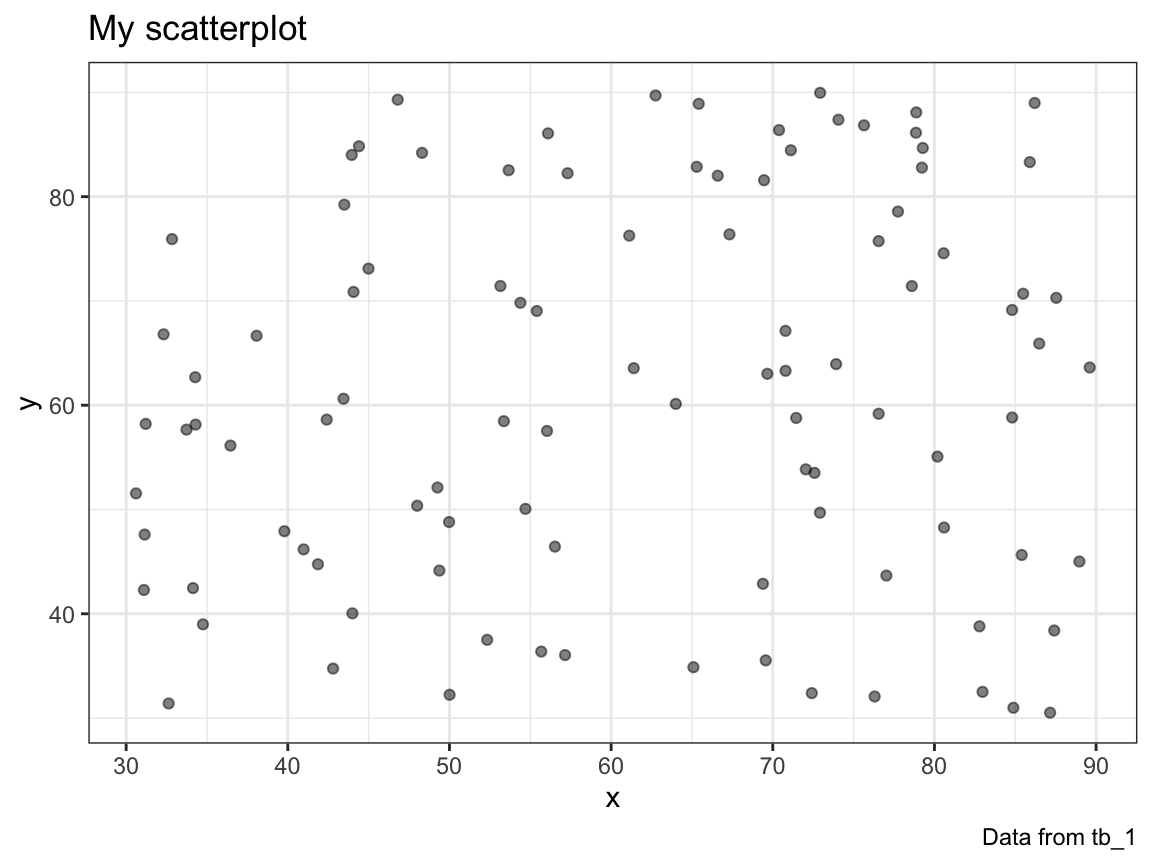
plot_scatter(my_data = tb_2)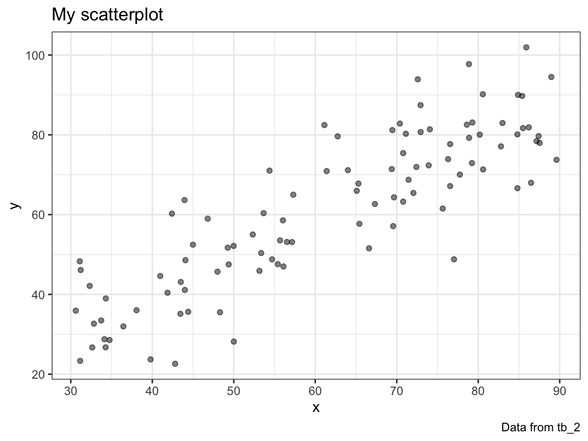
- For any table
my_datathat contains two numeric variablesxandywe can fit a linear model as follows:
my_data <- tb_1

my_lm <- lm(y ~ x, data = my_data)
my_lm
#>
#> Call:
#> lm(formula = y ~ x, data = my_data)
#>
#> Coefficients:
#> (Intercept)            x
#>     53.2340       0.1318

# Get the model's intercept and slope values:
my_lm$coefficients[1]  # intercept
#> (Intercept)
#>    53.23402
my_lm$coefficients[2]  # slope
#>         x
#> 0.1318431
Incorporate the fit of a linear model into your plot_scatter() function. Use a linear model to add a line to your plot that shows the prediction of the linear model (in a color that can be set by an optional col argument).
Solution
plot_scatter <- function(my_data, col = "red") {

  # fit linear model:
  lm <- lm(y ~ x, data = my_data)
  intercept <- lm$coefficients[1]
  slope <- lm$coefficients[2]

  # plot:
  ggplot(data = my_data) +
    geom_point(aes(x = x, y = y), alpha = 1/2, size = 2) +
    geom_abline(intercept = intercept, slope = slope, color = col, lty = 2, size = 1) +
    labs(title = "My scatterplot",
         caption = paste0("Data from ", deparse(substitute(my_data)))) +
    theme_bw()

}

# Check:
plot_scatter(my_data = tb_1, col = Pinky)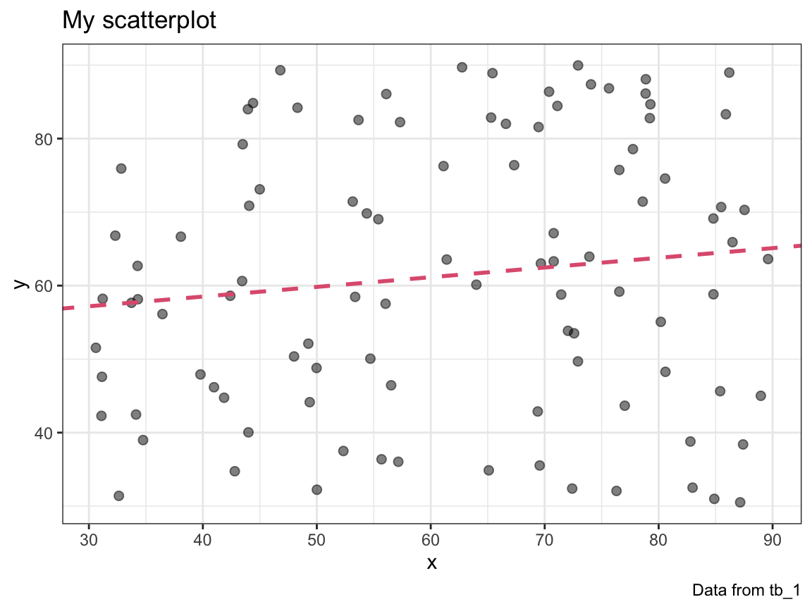
plot_scatter(my_data = tb_2, col = Seeblau)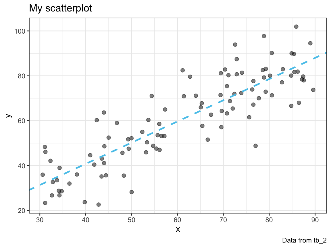
A.11.8 Exercise 8
Printing numbers (as characters)
A common problem when printing numbers in text is that the number of digits to be printed (i.e., characters or symbols) depends on the number’s value. This means that series of different numbers often have different lengths, which makes it hard to align them (e.g., in tables). A potential solution to this is adding leading or trailing zeros (or empty spaces) to the front and back of a number.
The function num_as_char() of the ds4psy package provides a (sub-optimal) solution to this problem by containing three main arguments:
xfor the number to be formatted (required);
n_pre_decfor the number of digits prior to the decimal separator (defaultn_pre_dec = 2);
n_decto specify the number of digits after the decimal separator (defaultn_dec = 2).
Additional arguments specify the symbol sym to use for filling up digit positions and the symbol used as decimal separator sep.
- Experiment with
num_as_char()to check its functionality and limits.
Solution
library(ds4psy)

# explore:
num_as_char(x =  1)
#> [1] "01.00"
num_as_char(x =  2, n_pre_dec = 3, n_dec = 3)
#> [1] "002.000"
num_as_char(x =  3.33, n_pre_dec = 1, n_dec = 1)
#> [1] "3.3"
num_as_char(x =  6.66, n_pre_dec = 1, n_dec = 1)  # rounding up
#> [1] "6.7"
num_as_char(x =  6.66, n_pre_dec = 2, n_dec = 0)  # rounding up
#> [1] "07"
num_as_char(x = 66.66, n_pre_dec = 1, n_dec = 1)  # not removing needed digits
#> [1] "66.7"

# limits:
num_as_char(1:4)   # works for vectors
#> [1] "01.00" "02.00" "03.00" "04.00"
num_as_char(1, sym = "89")  # works, but warns
#> [1] "891.8989"
# num_as_char(NA)  # yields an error
# num_as_char("X") # yields an error- Write your own function
num_to_char()that achieves the same (or a similar) functionality.
Hint: The ds4psy package contains a solution that also works for vectors, but uses two for loops to achieve this.
Try writing a simpler solution that works for individual numbers x (i.e., scalars, or vectors of length 1).
If you are stuck, try adapting parts of the solution used by num_as_char.
Solution
Evaluate ds4psy::num_as_char (without any parentheses) to inspect the (sub-optimal) solution implemented by the ds4psy package.
Then copy and adapt it for a simpler solution — by removing the for loops — that works for scalar numbers.
A.11.9 Exercise 9
Computing with dates
Use what you have learned in Chapter 10 on Dates and times to write a function that takes a date or time (e.g., the date of someone’s birthday) as its input and returns the corresponding individual’s age (as a number, rounded to completed years) as output.
Check your function with appropriate examples.
Does your solution also work when multiple dates or times are entered (as a vector)?
Solution
- Using only base R date and time functions:
# Define a function that computes current age (in full years):

age_in_years <- function(bdate){

  # Initialize:
  age <- NA

  # Assume that bdate is of class "Date" or "POSIXt".

  # Get some numbers:
  bd_year <- as.numeric(format(bdate, "%Y"))
  bd_month <- as.numeric(format(bdate, "%m"))
  bd_day <- as.numeric(format(bdate, "%d"))

  today <- Sys.Date()
  cur_year <- as.numeric(format(today, "%Y"))
  cur_month <- as.numeric(format(today, "%m"))
  cur_day <- as.numeric(format(today, "%d"))

  # # Determine whether bday happened this year:

  # # Non-vectorized version:
  # if ((cur_month > bd_month) || ((cur_month == bd_month) & (cur_day >= bd_day)))
  # {
  #   bday_this_year <- TRUE
  # }
  # else {
  #   bday_this_year <- FALSE
  # }

  # Vectorized version:
  bday_this_year <- ifelse((cur_month > bd_month) | ((cur_month == bd_month) & (cur_day >= bd_day)), TRUE, FALSE)

  # Compute age (in full years):
  age <- (cur_year - bd_year) - !bday_this_year

  return(age)

}
We check this function for some critical examples and a vector as input to bdate:
# Construct example:
today <- Sys.Date()    # today's date
today
#> [1] "2022-04-08"

N <- 100  # N of years
bday_1 <- today - (N * 365.25) - 1  # more than N years ago
bday_2 <- today - (N * 365.25) - 0  # exactly N years ago
bday_3 <- today - (N * 365.25) + 1  # less than N years ago

bday_1
#> [1] "1922-04-07"
bday_2
#> [1] "1922-04-08"
bday_3
#> [1] "1922-04-09"

age_in_years(bday_1)  # N
#> [1] 100
age_in_years(bday_2)  # N (after Feb 28 of a leap year)/1 (otherwise)
#> [1] 100
age_in_years(bday_3)  # N - 1 (qed)
#> [1] 99

# Testing limits:
# 1. age_in_years() also works for vectors:
bdays <- today - (N * 365.25) + -1:1
age_in_years(bdays)
#> [1] 100 100  99

# 2. age_in_years() works, but is not precise for (POSIXt) times:
sec_day <- (60 * 60 * 24)
btimes <- Sys.time() - (N * 365.25 * sec_day) + -1:1
age_in_years(btimes)
#> [1] 100 100 100- Using the lubridate package:
library(tidyverse)
library(lubridate)

lubriage <- function(bdate) {

  lifetime <- (bdate %--% today())  # time interval from bdate to today() OR now()
  (lifetime %/% years(1))           # integer division (into a period of full years)

}
Let’s also check this function for some critical examples and a vector as input to bdate:
# Construct example:
today()
#> [1] "2022-04-08"

N <- 100  # N of years
bday_1 <- today() - years(N) - days(1)  # N years ago, yesterday
bday_2 <- today() - years(N) + days(0)  # N years ago, today
bday_3 <- today() - years(N) + days(1)  # N years ago, tomorrow

lubriage(bday_1)  # N
#> [1] 100
lubriage(bday_2)  # N
#> [1] 100
lubriage(bday_3)  # N - 1 (qed)
#> [1] 99

# Testing limits:
# 1. lubriage() also works for vectors:
bdays <- today() - years(N) + days(-1:1)  # N years ago, -1/0/+1 days
lubriage(bdays)
#> [1] 100 100  99

# 2. lubriage() works, but is imprecise for times:
lubriage(btimes)
#> [1] 99 99 99
Let’s take a closer look at the last point:
- Do our functions also work for when entering times, rather than dates?
tnow <- now()  # current time
btimes_2 <- tnow - years(N) - seconds(6) + seconds(-1:1)  # N years ago, -1/0/+1 seconds

tnow      # current time
#> [1] "2022-04-08 17:04:09 CEST"
btimes_2  # N years ago + some seconds
#> [1] "1922-04-08 17:04:08 CET" "1922-04-08 17:04:09 CET"
#> [3] "1922-04-08 17:04:10 CET"

# Compare solutions:
age_in_years(btimes_2)
#> [1] 100 100 100
lubriage(btimes_2)
#> [1] 99 99 99
As we see, both functions appear to work with times. However, as they were not designed for them, their results may be wrong. In the present case, they actually yield different results. Which one would fit better to our common understanding of “How old are you today?” Thus, when creating new functions, we always need to consider the scope of their application.
Bonus task: Write alternative versions of the following lubridate functions:
a
my_leap_year()function (as an alternative tolubridate::leap_year()) that detects whether a givenyearis a leap year (see Wikipedia: leap year for definition).a
my_change_tz()function (as an alternative tolubridate::with_tz()) that converts the time display from its current time zone into a different one (tz), but keeping the point in time (i.e., the represented time) the same.a
my_change_time()function (as an alternative tolubridate::force_tz()) that changes a given time into the same nominal time (i.e., showing the same time display, but representing a different time) in a different time zone (tz).
Hints: See Section 10.3.4 of Chapter 10 for examples and the corresponding lubridate functions. Check your functions for a variety of examples and input types.
Solution
Compare and contrast your functions with the ds4psy functions is_leap_year(), change_tz(), and change_time():
# The ds4psy package implements (possibly imperfect) versions of these functions.

# To see the definition of a function "fun",
# evaluate ds4psy::fun (without parentheses):
ds4psy::is_leap_year

# or ?fun for the documentation of a function "fun":
?ds4psy::is_leap_year
Do your own functions accept the same inputs and yield the same outputs?
A.11.10 Exercise 10
A zodiac function
Use what you have learned in Chapter 10 on Dates and times to write a function that takes a date (e.g., the date of someone’s birthday) as its input and returns the corresponding individual’s zodiac sign (as a character or factor variable) as output.
Check your function with appropriate examples.
Does your function also work for vector inputs (containing more than one date)? What could be done to make it work for them?
Hints: This task may seem simple, but is quite challenging, for several reasons:
When working with dates in no particular year, we can treat them as character or numeric variables.
Basic conditionals in R only work for scalar inputs, not vectors. However, the base R function
cut()classifies continuous variables into discrete categories (see Section 11.3.7).Different sources provide different names and date ranges for the 12 zodiac signs. See https://en.wikipedia.org/wiki/Zodiac or https://de.wikipedia.org/wiki/Tierkreiszeichen for alternatives.
The ds4psy package also contains a zodiac() function that provides multiple output options and allows re-defining date ranges (see Table 11.2 for default settings).
| nr | name | from | to | symbol |
|---|---|---|---|---|
| 1 | Aries | 2022-03-21 | 2022-04-20 | ♈ |
| 2 | Taurus | 2022-04-21 | 2022-05-20 | ♉ |
| 3 | Gemini | 2022-05-21 | 2022-06-20 | ♊ |
| 4 | Cancer | 2022-06-21 | 2022-07-22 | ♋ |
| 5 | Leo | 2022-07-23 | 2022-08-22 | ♌ |
| 6 | Virgo | 2022-08-23 | 2022-09-22 | ♍ |
| 7 | Libra | 2022-09-23 | 2022-10-22 | ♎ |
| 8 | Scorpio | 2022-10-23 | 2022-11-22 | ♏ |
| 9 | Sagittarius | 2022-11-23 | 2022-12-21 | ♐ |
| 10 | Capricorn | 2022-12-22 | 2023-01-19 | ♑ |
| 11 | Aquarius | 2023-01-20 | 2023-02-18 | ♒ |
| 12 | Pisces | 2023-02-19 | 2023-03-20 | ♓ |
Solution
The implementation of zodiac() in the ds4psy package provides a possible solution that is quite flexible (but could be extended to include additional output formats).
Here are some examples that illustrates the function for a random sample of dates:
library(ds4psy)

dat <- sample_date(size = 10)
zod <- zodiac(dat)
sym <- zodiac(dat, out = "Unicode")

tab <- tibble::tibble(date = dat,
                      sign = zod,
                      symbol = sym)

knitr::kable(tab, caption = "Zodiac signs of 10 sampled dates.") | date | sign | symbol |
|---|---|---|
| 2000-02-25 | Pisces | ♓ |
| 1988-04-27 | Taurus | ♉ |
| 1988-09-24 | Libra | ♎ |
| 1992-05-12 | Taurus | ♉ |
| 1983-12-05 | Sagittarius | ♐ |
| 1993-07-02 | Cancer | ♋ |
| 1972-02-27 | Pisces | ♓ |
| 1970-11-26 | Sagittarius | ♐ |
| 1976-02-09 | Aquarius | ♒ |
| 1980-04-09 | Aries | ♈ |
This concludes our basic exercises on creating new functions. Section 11.7 contains additional exercises that address the more advanced topics of recursion and sorting.
Advanced exercises

The following more advanced exercises cover some topics introduced as Advanced aspects (in Section 11.4).
A.11.11 Exercise A1
Recursive arithmetic
Define some arithmetic operation (e.g., computing the sum, product, etc., of a vector) as a recursive function.
Solution
sum_rec()computes a vector sum in a recursive fashion:
sum_rec <- function(x) {

  if (length(x) == 1) {x}  # stop

  else { x[1] + sum_rec(x[-1]) }  # reduce & recurse

}

# Check:
sum_rec(1:4)
#> [1] 10
sum_rec(c(2, 4, 6))
#> [1] 12
sum_rec(1)
#> [1] 1
sum_rec(NA)
#> [1] NAinterest_rec()computes the compound interest (as a multiplicative factor) of a series of percentage valuespc_valin a recursive fashion:
pc_val <- c(2, 4, 6, -10)  # Series of percentage changes

prod((pc_val + 100)/100)   # arithmetic Solution
#> [1] 1.012003

pcf <- (100 + pc_val)/100  # as multiplicative factor

comp_interest_rec <- function(pcf) {

  if (length(pcf) == 0) {1}  # stop

  else { pcf[1] * comp_interest_rec(pcf[-1]) }  # reduce & recurse

}

# Check:
comp_interest_rec(pcf)
#> [1] 1.012003
A.11.12 Exercise A2
A rose is a rose…
Most illustrations of recursive functions address mathematical phenomena. As a non-numeric example, consider the literary phrase
“A rose is a rose is a rose is a rose.”
that is based on a poem by Gertrude Stein and became a popular meme (see flowery of the ds4psy package for 60 variants of the phrase).
The appeal of the phrase is largely due to its recursive aspect — so we should be able to use recursion to program a generator function for it.
Analysis:
- What part of the phrase is recursive? Which one is not?
- What is the stopping condition? What should happen when it is reached?
- What part of the phrase is recursive? Which one is not?
Write a recursive function
get_phrase(x = "rose", n = 3)that generates the phrase by repeating the partpaste0("is a", x)ntimes.- Note: It’s easy to write a function using repetition, but try writing a truly recursive function.
- Hint: Consider using an auxiliary function that only handles the recursive part of the phrase.
- Note: It’s easy to write a function using repetition, but try writing a truly recursive function.
Solution
get_phrase <- function(x = "rose", n = 3){

  out <- paste0("A ", x, get_recursion(x = x, n = n))

  return(out)

}

get_recursion <- function(x, n){

  if (n == 0) {s <- paste0(".")}

  else {

    s <- paste0(" is a ", x, get_recursion(x = x, n = n - 1))

  }

  return(s)

}

# Check:
get_phrase()
#> [1] "A rose is a rose is a rose is a rose."
get_phrase(n = 4)
#> [1] "A rose is a rose is a rose is a rose is a rose."
get_phrase("loop", 2)
#> [1] "A loop is a loop is a loop."
# Note:
get_phrase(n = 0)
#> [1] "A rose."
get_phrase(NA)
#> [1] "A NA is a NA is a NA is a NA."
A.11.13 Exercise A3
Solving the Towers of Hanoi (ToH)
The video clip Recursion ‘Super Power’ (in Python) by Computerphile explains how to recursively solve the Towers of Hanoi problem in Python:
- Watch the video and then solve the problem for \(n\) discs (e.g., by writing a function
ToH(n = 4)) in R.
Solution
# (A) Helper function: ----
move <- function(from, to){
  print(paste0("Move disc from ", from, " to ", to, "!"))
}

# Check:
move("A", "C")
#> [1] "Move disc from A to C!"


# # Not needed:
# move_via <- function(from, via, to){
#   move(from, via)
#   move(via, to)
# }
#
# # Check:
# move_via("A", "B", "C")


# (B) Main function: ----
ToH <- function(n, from = "A", helper = "B", to = "C"){

  if (n == 0) { NULL }  # stopping condition

  else { # solve simpler problems:

    ToH(n - 1, from = from, helper = to, to = helper)  # recursion 1

    move(from = from, to = to)  # move n-th disk

    ToH(n - 1, from = helper, helper = from, to = to)  # recursion 2

  }
}

# Check:
ToH(n = 4, from = "A", helper = "B", to = "C")
#> [1] "Move disc from A to B!"
#> [1] "Move disc from A to C!"
#> [1] "Move disc from B to C!"
#> [1] "Move disc from A to B!"
#> [1] "Move disc from C to A!"
#> [1] "Move disc from C to B!"
#> [1] "Move disc from A to B!"
#> [1] "Move disc from A to C!"
#> [1] "Move disc from B to C!"
#> [1] "Move disc from B to A!"
#> [1] "Move disc from C to A!"
#> [1] "Move disc from B to C!"
#> [1] "Move disc from A to B!"
#> [1] "Move disc from A to C!"
#> [1] "Move disc from B to C!"
#> NULL
Use your
ToH()function for solving then = 3case and answer the following questions:How many disc moves does this require?
How often does the function meet the stopping criterion (i.e.,
n == 0)?
Hint: To determine this, you could print out “ok” (or some counter value) every time you reach this condition.
Solution
# (B2) Variant of ToH (with "ok" at stopping condition): ----
ToH_ok <- function(n, from = "A", helper = "B", to = "C"){

  if (n == 0) { print("ok") }  # stopping condition with "ok"

  else { # solve simpler problems:

    ToH_ok(n - 1, from = from, helper = to, to = helper)  # recursion 1

    move(from = from, to = to)  # move n-th disk

    ToH_ok(n - 1, from = helper, helper = from, to = to)  # recursion 2

  }
}

# Check:
ToH_ok(3)
#> [1] "ok"
#> [1] "Move disc from A to C!"
#> [1] "ok"
#> [1] "Move disc from A to B!"
#> [1] "ok"
#> [1] "Move disc from C to B!"
#> [1] "ok"
#> [1] "Move disc from A to C!"
#> [1] "ok"
#> [1] "Move disc from B to A!"
#> [1] "ok"
#> [1] "Move disc from B to C!"
#> [1] "ok"
#> [1] "Move disc from A to C!"
#> [1] "ok"- The solution shown in the video provides a recipe for solving the problem, but does not explicate which disc is being transferred on each move.
Slightly adjust themove()helper function and its call in theToH()function so that the disc being transferred is identified by its sizen(withn = 1denoting the smallest disc, andn = ndenoting the largest disk).
Solution
# (A) Adjusted helper function: ----
move_n <- function(n, from, to){

  print(paste0("Move disc ", n, " from ", from, " to ", to, "!"))

}

# Check:
move_n(123, "A", "C")
#> [1] "Move disc 123 from A to C!"


# (B) Adjusted main function: ----
ToH <- function(n, from = "A", helper = "B", to = "C"){

  if (n == 0) { NULL }  # stopping condition

  else { # solve simpler problems:

    ToH(n - 1, from = from, helper = to, to = helper)  # recursion 1

    move_n(n = n, from = from, to = to)  # move n-th disk

    ToH(n - 1, from = helper, helper = from, to = to)  # recursion 2

  }
}

# Check:
ToH(n = 3, from = "A", helper = "B", to = "C")
#> [1] "Move disc 1 from A to C!"
#> [1] "Move disc 2 from A to B!"
#> [1] "Move disc 1 from C to B!"
#> [1] "Move disc 3 from A to C!"
#> [1] "Move disc 1 from B to A!"
#> [1] "Move disc 2 from B to C!"
#> [1] "Move disc 1 from A to C!"
#> NULL
A.11.14 Exercise A4
More sorting and measuring
- Watch the following video clip and implement at least one sorting algorithm not yet illustrated in this chapter as an R function.
- 15 Sorting Algorithms in 6 Minutes (by Timo Bingmann): Visualization and “audibilization” of 15 sorting algorithms in 6 minutes. Sorts random shuffles of integers, with both speed and the number of items adapted to each algorithm’s complexity.
- Compare the performance of your new function with those discussed in Section 11.4.2 on a suitable range of problems.
This concludes the more advanced exercises on programming in R.