1.2 Data vs. functions
To understand computations in R, two slogans are helpful:
- Everything that exists is an object.
- Everything that happens is a function call.John Chambers
R is a programming language, but learning R is also a bit like stepping into a new galaxy or acquiring a new superpower. Unfortunately, both galaxies and superpowers tend to be a bit overwhelming at first. This struggle must not turn into an outright battle (though I could not resist the analogy of Figure 1.3), but understanding a few basic concepts helps a lot in staying oriented during our explorations.

Figure 1.3: Learning R involves not just a new language, but navigating a galaxy of objects. Some of them are atoms, but functions are stars. Understanding and using functions is the force that will guide us through our battles of the Rwars legacy. (Image created by using the R package meme.)
In R, we mostly need to grasp the notions of objects and functions. From a task-oriented perspective, using R and most other programming languages consists in
- creating or loading data (inputs, material, values), and
- calling or evaluating functions (actions, verbs) for
- computing and constructing new data (outputs, images, tables, results).
Confusingly, both data and functions in R are objects (stuff) and evaluating functions typically returns or creates new objects (more stuff). Thus, the process of computation can be viewed as a cycle that uses data (as input) to create more data (as output). Although any part of a program is an object, functions are those objects that do things by processing and creating new objects. To distinguish data from functions, think of data as matter (i.e., material, stuff, or values) that are being measured, manipulated, or processed, and of functions as procedures (i.e., actions, operations, or verbs) that measure, manipulate, or process data. Put more succinctly, functions are objects that do things — they process data into other data.
Although this chapter addresses data and functions in the context of base R, the same distinctions also apply to other packages and languages. In the following, we will introduce some ways to describe data (by shape and type), learn to create new data objects (by assigning them with <-), and apply some pre-defined functions to these data objects.
A note on notation
To make it easier to distinguish between data objects and functions in this book, we will typically add (round) parentheses to function names. Thus, c() indicates a function, whereas c indicates a data object — and c[] is yet another thing (see below).
However, we may sometimes forget or forgo this convention when it is clear that an object foo is the function foo().
Additionally, there exist some R functions that work without parentheses (e.g., arithmetic operators + and * that are positioned between their arguments).
As R functions also are objects, they can even be the inputs and outputs of functions. Thus, the difference between functions and data objects is helpful, but primarily matters in the user’s mind.
1.2.1 Data objects
A primary goal of data science is to gain insights and draw conclusions from analyzing the content and context of data (e.g., the meanings implied by some measurements). However, before we can begin to create and use any data objects in R, it is helpful to reflect on the difference between data and information, distinguish between variables and values, and view data objects in terms of their shape and type.
Data vs. information
Data must not be confused with information. Without getting too technical, data is the raw material of information, but needs to make sense (by being structured and becoming useful) to be informative. Taken literally, the term data merely is the plural of a singular datum, which is a Latin term for something given.
According to Wikipedia, data “are characteristics or information, usually numerical, that are collected through observation.” This definition sounds a little fishy. While not technically false, it is vague and emphasizes numerical data over non-numeric data. The following definition (also from Wikipedia) is more precise, but introduces additional terms:
“In a more technical sense, data are a set of values of qualitative or quantitative variables about one or more persons or objects, while a datum (singular of data) is a single value of a single variable.”
This sounds smart and may even be true, but the trick here is to delegate the definition to related concepts and hope that the person asking the original question will give up: If data are the values of variables, what are those?
The key to understanding the nature of data lies in realizing that data is a representation with an intentional structure:
Some sign or symbol (e.g., a number and unit of measurement) denotes something else — typically some aspect of the world.
For instance, some data point \(10m\) can represent the height of a tree and is typically the result of some observation (measurement or estimation).
Such observations can be expressed as verbal statements (e.g., “The height of this tree is \(10m\)”) or in formal notation (height(tree) = 10), which can further characterized as being accurate/inaccurate, or TRUE/FALSE.
Data shapes vs. types
When formally dealing with data, it makes sense to distinguish between a variable and its values:
A variable is a dimension or property that describes a unit of observation (e.g., a person) and can typically assume different values.
By contrast, values are the concrete instantiations that a variable assigns to every unit of observation and are further characterized by their range (e.g., categorical vs. continuous values) and their type (e.g., logical, numeric, or character values).
For instance, an individual can be characterized by the variables name, age, and whether or not s/he is classified as an adult.
The values corresponding to these variables would be of type text (e.g., “Lisa”), numeric (e.g., age in years), and logical (TRUE vs. FALSE, defined as a function of age).
In scientific contexts, variables are often defined as numeric measures and computed according to some rule (e.g., by some mathematical formula) from other variables. For instance, the positive predictive value (PPV) of a diagnostic test is a conditional probability \(P(TP|T+)\) that can be computed by dividing the test’s hits (e.g., the frequency count of true positive cases, \(TP\)) by the total number of positive test outcomes (\(T+\)). Given its definition (as a probability), the range of values for the variable PPV can vary continuously from 0 to 1.
In R, data is stored in objects that are distinguished by their shape and by their type:
The most common shapes of data are:
- scalars are individual elements (e.g.,
"A",4,TRUE);
- vectors are linear chains or sequences of objects (of some length);
- tables are rectangular data structures with two dimensions (with rows and columns).
- scalars are individual elements (e.g.,
The most common types of data are:
- logical data (for representing truth values of type
logical, aka. Boolean values);
- numeric data (for representing numbers of type
integerordouble);
- text data (for representing text data of type
character);
- time data (for representing dates and times).
- logical data (for representing truth values of type
There are additional data shapes (e.g., multi-dimensional data structures) and types (e.g., for representing categorical or geographical data), but the ones mentioned here are by far the most important ones. Due to technical aspects of R, we can further distinguish between an object’s an object’s type, it’s mode, and it’s class, but these details is irrelevant at this point.
When simultaneously considering the shape and type of data, we can distinguish and begin to understand data structures.
Data structures in R
Data structures are constructs designed to store data. As we mentioned in Section 1.1.3, the data structures of a programming language are similar to the grammatical and spelling rules of natural languages. As long as we reach our goals, we neither care about nor need to know the rules. But whenever unexpected outcomes or errors occur, repairing them in a competent fashion requires considerable background knowledge and experience.
Although the term “data structure” is sometimes used to refer to just the shape of data, understanding the key data structures available in R requires viewing them as a combination of (a) some data shape, and (b) the fact whether they contain a single or multiple types of data.
Table 1.1 provides an overview of the key data structures provided by the designers of R. Note that Table 1.1 distinguishes between three different data shapes (in its rows) and between data structures for “homogeneous” vs. “heterogeneous” data types (in its columns):
| Dimensions: | Homogeneous data types: | Heterogeneous data types: |
|---|---|---|
| 1D | atomic vectors: vector |
list |
| 2D | matrix |
rectangular tables: data.frame/tibble |
| nD | array/table |
Although Table 1.1 contains entries for five different shape-type combinations of data structures, two of them are by far the most important data structures from the perspective of R users:
atomic vectors are linear data structures that are characterized by their length and type (mode or class). Crucially, vectors only extend in one dimension (i.e., their length) and only contain a single type of data.16
rectangular tables are tabular data structures that extend in two dimensions (rows and columns). As a
matrixalso is a rectangle of data, the defining feature of rectangular tables is not their shape, but the fact that they can store data of different types (e.g., variables of type character, logical values, and numbers). The technical termsdata.frameandtibbledenote two slightly different variants of such tables.
The overview provided by Table 1.1 will become much clearer after seeing some examples of each data structure. Crucially, the key to understanding Table 1.1 lies in viewing data structures as a combination of data types and data shapes. Whereas the different data shapes (linear, rectangular, n-dimensional) are usually quite obvious, the distinction between homogeneous and heterogeneous data types is more subtle. Note that the combination “heterogeneous data types” only implies that such structures can store different types of data, and that the corresponding data structures (i.e., lists and rectangular tables) are also described as “hierarchical” or “recursive.”
Relations between data structures
Note that the different shape-type combinations in Table 1.1 are not independent of each other.
In terms of its implementation, a matrix is actually a vector with two additional attributes (i.e., the number of rows and columns) that determine its shape, or a 2-dimensional instance of an array.
Technically, even lists are implemented as vectors in R, but in contrast to atomic vectors, lists are so-called “recursive vectors.”
And as lists are R’s data structure for accommodating heterogenous types of data, rectangular tables are implemented as lists of atomic vectors that all have the same length. Thus, from the perspective of developers, there are two main data structures in R: vectors and lists.
A good question is: Where are scalar objects in Table 1.1? The answer is: R is a vector-based language. Thus, even scalar objects are represented as (atomic, i.e., homogeneous) vectors (of length \(1\)).
When introducing data structures in more detail, we will progress from simpler shapes to more complex ones, by first defining scalars (Section 1.3), before moving on to vectors (Section 1.4), rectangular tables (Section 1.5), and lists (Section 1.6.3). But before learning to create and use these structures, we will contrast data objects with another type of object: In R, functions are active objects (or commands) that do stuff with data objects.
Practice
Our description of Table 1.1 stated that the most important shape-type combinations are atomic vectors and rectangular tables. But only a few lines later, its was also stated that the two main data structures in R are vectors and lists. Is this not a conflict or contradiction? Discuss and explain.
What are the consequences of designing rectangular tables as lists of columns (rather than lists of rows) for their interpretation?
Solution
ad 1.: There is no conflict, and the apparent contradiction is dissoved when distinguishing between two different perspectives:
R users can typically solve their tasks by knowing only vectors (for storing one type of data) and rectangular tables (for storing data of different types). These two combinations of data shapes and types hit the sweet spots in terms of simplicity, flexibility, and practical usefulness.
By contrast, R designers and programmers need to also consider the implementation of data structures: Vectors and lists are the two main building blocks for homogeneous vs. heterogeneous types of data. For instance, rectangular data structures that store heterogeneous types of data are implemented as lists.
ad 2.: Whereas vectors can only store data of a single data type (e.g., only numbers or only text characters), we typically want rectangular tables to allow for data of multiple types (e.g., character and numeric variables). In principle, both a by-row and a by-column organization would be possible when creating a rectangular table. However, the creators of R opted for a by-column organization and designed a rectangular table as a list: Each list element is a vector (i.e., a column/variable of only one type of data). Thus, each row of the resulting table is a case or observation (i.e., describes an individual on multiple variables).
1.2.2 Creating objects
To create a new object in R, we determine its name and its value and then type and evaluate an assignment expression of the form:
name <- value
For instance, assuming that we want to create a simple object named “x” and assign it to a numeric value of 1, we would type and evaluate:
x <- 1Evaluating this expression creates a new object x with a numeric value of 1.
An alternative way of achieving the same assignment would be:
x = 1Although using = works and may be more familiar from mathematics, using the assignment operator <- is the preferred way of creating objects in R.17
More generally, to create an object o and initialize it to v, we type and evaluate an expression of the form o <- v. Importantly, v can be another R expression. For instance, we can assign the output of a function to a new object s:
s <- sum(1, 2)What kind of object s did we just create?
While this may easily be guessed, it is quite challenging to express everything that happened in this line of code in appropriate words.
A good answer would require a number of technical terms that are defined and used in this chapter:
This R expression creates a new object s by assigning it to the result of sum(2, 3).
The expression sum(1, 2) to the right of the assignment operator is a function with two numeric arguments (1 and 2).
When R evaluates the assignment, it first computes the result of sum(1, 2) and then assigns it to an object s.
Interestingly, evaluating s <- sum(1, 2) may have done all this, but did not yield any obvious result.
To examine s, we need to remember that doing anything in R requires a function (or “everything that happens is a function call”).
1.2.3 Using objects
Using an R object implies (a) that it exists (i.e., has been created), and (b) that its name appears in some function that is evaluated.
Perhaps the simplest function to be applied to an object is print():
print(s)
#> [1] 3
which can be abbreviated by:
s
#> [1] 3
When R evaluates print(s) (or the line of code in which it occurs) the content (or value) of object s is printed (as 3).
Although all this may not be too surprising, note that we have already learned at least three things about R:
- how to create objects
- how to evaluate functions
- how to print (the contents of) an object
To complete this achievement, note that all this can be achieved in one line:
(s <- sum(1, 2))  # assign and print(s)
#> [1] 3
Enclosing an assignment in (round) parentheses assigns an object (to the result to the right of the assignment operator <-) and immediately prints it.
As our new object s is a numeric object (with a value of 3), we can apply simple arithmetic functions to it:
s + 2
#> [1] 5
s^2
#> [1] 9
Note that R saves us the trouble of explicitly printing the results. For many functions, the results are immediately printed when evaluating the function.
Here is another example of creating two basic objects by assigning numeric values to them:
# Creating objects:
o <- 10  # assign/set o to 10
O <-  5  # assign/set O to  5
As R is case-sensitive, o and O denote two different objects (even if the same number was assigned to both).
As the two objects just created also were numeric objects, we can apply more arithmetic functions to them:
# Computing with objects:
o * O
#> [1] 50
o * 0  # Note: O differs from 0
#> [1] 0
o / O
#> [1] 2
O / 0
#> [1] Inf
As explained in Section 1.2.1, R data objects are stored in data structures, which are characterized by the shape (i.e., length or dimensions) and type of the object (see Table 1.1, for an overview).
When defining an object, we can always ask three questions:
What is the type of this object?
What shape does it have?
What data structure is used to store this object?
With respect to the four objects defined in this section (i.e., x, s, o, and O), the answers to these questions are as follows:
The data type all objects is
numeric.18The shape of each object is a linear sequence of length 1.
The data structure used to store each of them is a vector.
The essential aspects can be summarized as follows:
The type of an object mostly corresponds to the type of data that has been assigned to the object. The simplest data structures only contain a single type of data (e.g.,
numeric,character, orlogical), but more complex data structures (e.g., data structures that are of typelistordata.frame) can contain multiple data types.Most R users primarily deal with two shapes of objects:
Linear objects are 1-dimensional data structures that collect zero to many elements. Linear objects with a length of 1 are called scalars, longer linear objects are either vectors (when only containing one type of data) or lists (when containing several types of data).
Rectangular tables are 2-dimensional data structures that can store data of several types. Internally, they are implemented as lists of vectors.
Practice
- Given the current definitions of this section, explain the meanings of the following expressions, and predict their results:
x
x + o
o + O
x <- O
x + o- Check your predictions by evaluating the expressions.
Solution
The results (when evaluating the five expressions from top to bottom) are:
#> [1] 1
#> [1] 11
#> [1] 15
#> [1] 15
Given that a simple assignment like o <- 10 achieved an awful lot (i.e., create a new data structure to store an object o with a specific shape and type), a reasonable question are:
How can we check (examine or test for) the characteristics of an object?
How do we change an object?
Checking objects by generic functions
The answer to Question 1 is straightforward:
- To check (examine or test) an object, we apply generic functions to it.
We know that doing anything in R requires functions. As different functions solve different tasks, we need to ask different functions to answer different questions. So the tricky term here is the word “generic.” A generic function is simply a function that can be applied to most or all R objects.
Here are some examples of generic functions that check an object’s shape, type, and data structure:
# Checking an object (by generic functions):

# A: Object shape:
length(o)
#> [1] 1
# dim(o)

# B: Object type:
mode(o)
#> [1] "numeric"
typeof(o)
#> [1] "double"

is.numeric(o)
#> [1] TRUE
is.character(o)
#> [1] FALSE
is.logical(o)
#> [1] FALSE

# C: Data structure:
is.vector(o)
#> [1] TRUE
is.list(o)
#> [1] FALSE
Changing objects by re-assigning them
Question 2 (i.e., how to change existing objects) can be asked more specifically:
- How do we change the shape, type, or data structure of an object?
The answer to these questions could hardly be any simpler:
- To change an object, we simply re-create (i.e., re-assign) it with a different definition.
Importantly, re-assigning an object can change all its characteristics.
For instance, we can change an object by re-assigning it to a different value:
# Re-assigning o:
(o <- 100)
#> [1] 100

# Check object:

# shape:
length(o)
#> [1] 1

# type:
mode(o)
#> [1] "numeric"
typeof(o)
#> [1] "double"

is.numeric(o)
#> [1] TRUE
is.character(o)
#> [1] FALSE
is.logical(o)
#> [1] FALSE

# data structure:
is.vector(o)
#> [1] TRUE
is.list(o)
#> [1] FALSE
The result of these generic functions show that reassigning the object o (from o <- 10 to o <- 100) merely changed its value, but not its shape, type, or the data structure used to store it.
This changes when we re-assign a different type of object to o:
# Re-assigning o:
(o <- c("A", "B", "C"))
#> [1] "A" "B" "C"

# Check object:
length(o)
#> [1] 3

mode(o)
#> [1] "character"
typeof(o)
#> [1] "character"

is.vector(o)
#> [1] TRUE
is.list(o)
#> [1] FALSE

is.numeric(o)
#> [1] FALSE
is.character(o)
#> [1] TRUE
is.logical(o)
#> [1] FALSE
In this case, we re-assigned o to an atomic vector (i.e., a linear data structure that only allows for one data type).
The particular vector here was of type character and had a length of three elements.
Thus, this re-assignment changed several characteristics of o. In fact, it simply created a new object o with quite different characteristics. The important lession to remember is:
- To change an object, we simply re-create (i.e., re-assign) it with a different definition.
Practice
- Change
oto the result of the arithmetic expression1 > 2and examine the resulting object by generic functions:
# Re-assign o:
o <- 1 > 2
o  # print(o)

# Check object:
length(o)

mode(o)
typeof(o)

is.vector(o)
is.list(o)

is.numeric(o)
is.character(o)
is.logical(o)- Although the difference between the mode and type of an object is not very important (in this chapter), note for which versions of object
othe generic functionsmode(o)andtypeof(o)yielded different results.
Solution
The results of mode(o) and typeof(o) only differed when assigning numbers to o.
In these cases, the object’s mode was numeric and its type double.
By contrast, the generic mode() and typeof() functions showed no difference when o was of type character or logical.
1.2.4 Naming objects
An important aspect of working with R consists in creating and naming new objects. Finding good names for data objects and functions is key for writing transparent code, but can often be challenging, especially as our understanding of a topic changes over time.
Rules
When naming new objects, beware of the following characteristics and constraints:
R is case sensitive (so
tea_pot,Tea_potandtea_Potare different names that would denote three different objects);Avoid using spaces inside variables (even though names like
'tea pot'are possible);Avoid special keywords that are reserved for R commands (e.g.,
TRUE,FALSE,function,for,in,next,break,if,else,repeat,while,NULL,Inf,NaN,NAand some variants likeNA_character,NA_integer, …).
Recommendations
Naming objects is partly a matter of style, but clarity and consistency are always important. Sensible recommendations for naming objects include:
Always aim for short, clear, and consistent names. Helpful suggestions include:
- Names of simple numbers should be simple and relate meaningfully to each other (e.g.,
xandyfor coordinates,ivs.jfor indices, etc.); - Names of data objects should indicate their shape (e.g.,
vfor vector,dffor data frames);
- Names of functions should indicate what they do (i.e., the task they solve, their purpose/function).
- Names of simple numbers should be simple and relate meaningfully to each other (e.g.,
Avoid dots and special symbols (e.g., spaces, quotes, etc.) in names (unless you are programming methods for R classes);
Consistently use either
snake_case(with underscores) orcamelCase(with capitalized first letters) for combined names;Avoid lazy shortcuts like
TforTRUEandFforFALSE. They may save a few milliseconds when typing a value, but can cause terrible confusion when someone happens to assignT <- 0orF <- 1somewhere.
Practice
Naming rules and recommendations are often ridiculed and even more frequently violated. To understand that good names are useful, reflect on the following examples:
- In R, the function
c()combines or concatenates elements into a vector. Predict and explain the result of:
c <- 1
c(c)- A seemingly innocuous assignment can wreak logical havoc when being lazy with logical values:
F <- 1

T & F   # is TRUE
T == F  # is TRUE
T != F  # is FALSE
We will encounter additional examples of (deliberate) bad naming when exploring functions and in Exercise 2 (see Section 1.2.6 and 1.8.2 below).
1.2.5 Function objects
Function objects are usually just called “functions,” but the clumsy term “function objects” makes it clear that functions are also defined as objects in R. As we will only begin to define our own functions in Chapter 11, we first learn to use a large variety of functions provided by base R and other packages.
When data objects serve as the elementary ingredients of computer programming, function objects are active operators (or verbs) that use and transform data. Without functions, nothing would ever happen in R — and our data would just passively sit around and never change. Thus, think of functions as ‘action operators’ that are applied to ‘data objects.’
In R, a function named foo is “called” by specifying the function’s name (i.e., foo) and appropriate data objects as its so-called arguments (e.g., a1 and a2). Function arguments are enclosed in (round) parentheses and best specified in a name = value notion, as in:
# Calling a function:
foo(a1 = 1, a2 = 2)
A function is an instruction or a process that takes one or more data objects (e.g., two arguments a1 and a2) as input and converts them into some output (i.e., an object that is returned by the function).
The function’s name, and the names, nature, and number of its inputs and outputs varies by its purpose.
An example of a simple function that accepts two numeric arguments is sum():
sum(1, 2)
#> [1] 3
Here, the function sum() is applied to two numeric arguments 1 and 2 (but note that we did not specify any argument names).
Evaluating the expression sum(1, 2) (e.g., by entering it into the Console and pressing “Enter/return,” or pressing “Command + Enter/return” within an expession in an R Editor) returns a new data object 3, which is the sum of the two original arguments.
Terminology
As functions are instructions for turning input into output, they are also referred to as commands. The combination of a function (i.e., an action object) and its arguments (i.e., the data objects serving as its inputs) is often called an expression or a statement. Such expressions or statements can be called or evaluated to return a result (i.e., another data object that is returned as the function’s output).
As functions are our main way of analyzing and transforming data, understanding and distinguishing between these terms is helpful and important. The following code chunk summarizes this function-related terminology:
# Explore the "function"/"command" named "sum":
sum(1, 2)  # An "expression" or "statement" to be evaluated:
# sum() uses 2 "arguments": 1, 2 (a numeric data objects, as inputs)
# ==> returns the "result":    3 (a numeric data object, as output)
Practice
Describe and evaluate the following expression:
sum(c(1, 2))What kind of object is
c()?What does the expression return when evaluated?
What does the result imply for the
sum()function?
Solution
Even without knowing the meaning of
c(), the round parentheses indicate that it is a function named “c.”Evaluating the expression
sum(c(1, 2))in R returns the numeric object 3, just like evaluatingsum(1, 2)did.The expression
sum(c(1, 2))calls thesum()function on the result of thec()function with two numeric arguments 1 and 2. If the result ofc(1, 2)is a data object, then thesum()function can also be evaluated for a single argument. (In Section 1.4.2, we will learn that the expressionc(1, 2)creates a data object known as a vector. This vector is a data object with two numeric elements 1 and 2.)
Using vs. creating functions
We could only use (i.e., call and evaluate) the expressions sum(1, 2) and sum(c(1, 2)) because R comes pre-equipped and pre-loaded with a range of basic functions.
Learning to use the functions existing in base R and other R packages is the key task that will pre-occupy us for the first weeks or months of our data science career.19
As mentioned above, we will eventually learn to create (i.e., write or program) our own functions (in Chapter 11). However, even experienced R programmers spend the majority of their time by using, searching for, and exploring existing functions. Once we have written some useful new functions, we can collect and share them with other users by writing an R package.
Functions as data
The useful distinction between data and functions made here should not tempt us to think that these concepts are mutually exclusive (i.e., that any object either is data or a function). An advanced aspect of R is that functions can be used as data (e.g., passed as arguments to other functions). We will later encounter this phenomenon under the label of functional programming (in Section 12.3). At this point, however, it is sufficient to view data as “passive” objects and functions as “active” objects.
Practice
Let’s explore some base R functions in various ways:
- What does the function
sum()do? How many and which types of arguments does it accept?
Hint: Explore some examples first, then study the function’s documentation by entering ?sum into the Console.
# Arguments of sum():
sum(1)
sum(1, 2)
sum(1, 2, 3)
sum(1, 2, 3, NA)
sum(1, 2, 3, NA, na.rm = TRUE)
sum(1:100)- Evaluate the following expressions (i.e., functions with arguments) and try to describe what they are doing (in terms of applying functions to data arguments to obtain new data objects):
# Functions with numeric arguments:
sum(1, 2, -3, 4)
min(1, 2, -3, 4)
mean(1, 2, -3, 4)
sqrt(121)

# Functions with characters as arguments:
paste0("hell", "o ", "world", "!")
substr(x = "television", start = 5, stop = 10)
isTRUE(2 > 1 & nchar("abc") == 4)
Obtaining help and omitting argument names
Using R typically involves using many different functions. Whenever we encounter an unfamiliar function, studying the function’s online documentation can be very helpful (even though it may take some practice to appreciate this).
To obtain help on an existing function, you can always call ? and the name of the desired function. For example:
# Note: Evaluate
?substr
# to see the documentation of the substr() function.
The argument names of functions can be omitted. When this is the case, R assumes that arguments are entered in the order in which they appear in the function definition. When explicitly mentioning the argument names, their order can be switched. Thus, the following function calls should all evaluate to the same results:
# Ways of calling the same function:
substr(x = "television", start = 5, stop = 10)
substr("television", 5, 10)
substr(start = 5, x = "television", stop = 10)
Hint: Omitting argument names is convenient when evaluating functions on the fly. However, in longer programs and especially when writing code that is read and used by others, it is better to spell out argument names (for explication and documentation purposes).
Practice
Let’s practice some additional inspections of and interactions with functions:
Retrieve the documentation for the
sum()function (by evaluating?sum):- Where does the documentation show which R package this function belongs to?
- Which arguments does the function accept?
- Evaluate the Examples provided by the documentation.
What happens when we ask for the documentation of the
filter()function?- Which packages define a
filter()function?
- Which packages define a
Hint: Different R packages can define the same functions.
To refer to a function defined by a particular package pkg, you can precede the function by pkg::.
?filter  # 2 different packages define a function of this name

# Indicating the filter() function of a particular package:
?stats::filter
?dplyr::filter- Try predicting the outcome of
substr("television", 20, 30)(e.g., by studying its documentation). Then check your prediction by evaluating it, studying the function’s documentation, and evaluating some variants.
substr("television", 20,  30)

# online documentation:
?substr

# variants:
substr(x = "television", start = 1, stop = 30)
substr("television", 1,  4)
substr("television", 9, 99)
substr("abcdefg", 4, 6)
1.2.6 Exploring functions
Exploring new functions is an important skill when dealing with a functional programming language like R. We can think of a function as a black box that accept certain inputs (called arguments) and transform them into outputs. Understanding a new function aims to map the relation between inputs and outputs. Importantly, we do not need to understand how the function internally transforms inputs into outputs. Instead, adopting a “functional” perspective on a particular function involves recognizing
its purpose: What does this function do? What inputs does it take and what output does it yield?
its options: What arguments does this function provide? How do they modify the function’s output?
In the following, we will explore both a simple and a more complex function to illustrate how functions can be understood by studying the relation between their inputs and outputs.
Exploring a simple function
Many functions are almost self-explanatory and relatively easy to use, as they require some data and offer only a small number of arguments that specify how the data is to be processed. Ideally, the name of a function should state what it does.
An example of such a straightforward function is the sum() function, which — surprise, surprise — computes the sum of its arguments:
sum(1, 2, -3, 4)
#> [1] 4
This seems trivial, but evaluating ?sum reveals that sum() also allows for an argument na.rm that is set to the logical value of FALSE by default.
This arguments essentially asks “Should missing values be removed?”
To see and understand its effects, we need to include a missing value in our numeric arguments.
In R, missing values are denoted as NA:
# Calling the function with its default value for na.rm:
sum(1, 2, -3, NA, 4)
#> [1] NA

# This is the same as:
sum(1, 2, -3, NA, 4, na.rm = FALSE)
#> [1] NA

# Note the difference, when na.rm is set to TRUE:
sum(1, 2, - 3, NA, 4, na.rm = TRUE)
#> [1] 4
These explorations show that sum() normally yields a missing value (NA) when its arguments include a missing value (NA), as na.rm = FALSE by default.
To instruct the sum() function to ignore or remove missing values from its computation, we need to specify na.rm = TRUE.
Exploring a complex function
Learning to use a more complex function is a bit like being presented with a new toy that comes with many buttons: What happens when we push this one? What if we combine these two, but not this other one? Given the ubiquity of functions in R, understanding how they work is an important skill. Experienced programmers often face a choice between finding and using someone else’s function (that someone surely has written somewhere at some time) and writing your a new function. (We will learn to write our own functions in Chapter 11.)
Exploring unfamiliar functions can be fun — and actually is a bit like conducting empirical research: As functions typically are systematic systems, we can test hypotheses about the effects of their arguments. And discovering the systematic properties of a system can be entertaining and exciting.
To demonstrate this process, the ds4psy package contains a function plot_fn() that — for illustration purposes — intentionally obscures the meaning of its arguments. In the following, we will explore the plot_fn() function to find out what its arguments do.
Explore the function by entering the following commands. But beware: As the plot_fn() function contains some random elements, your outputs may differ from the ones shown here. Thus, the challenge of understanding the function lies in discovering its systematic elements above and beyond its random ones.
Loading the package and evaluating the plot_fn() with its default arguments yields the following:
library(ds4psy)  # load the package
plot_fn()
It seems that the function plots colored squares in a row. However, calling it repeatedly yields a varying number of squares — this reveals that there is some random element to the function. When entering plot_fn() in the editor or console, placing the cursor within the parentheses (), and hitting the Tab key of our keyboard (within the RStudio IDE) we see that plot_fn() accepts a range of arguments:
xA (natural) number. Default:x = NA.yA (decimal) number. Default:y = 1.ABoolean. Default:A = TRUE.BBoolean. Default:B = FALSE.CBoolean. Default:C = TRUE.DBoolean. Default:D = FALSE.EBoolean. Default:E = FALSE.FBoolean. Default:F = FALSE.fA color palette (e.g., as a vector). Default:f = c(rev(pal_seeblau), "white", pal_pinky). Note: Using colors of the unikn package by default.gA color (e.g., as a character). Default:g = "white".
Calling a function without arguments is the same as calling the function with its default arguments (except for random elements):
plot_fn()  # is the same as calling the function with its default settings:
plot_fn(x = NA, y = 1, A = TRUE, B = FALSE, C = TRUE, D = FALSE, E = FALSE, F = FALSE)
# (except for random elements).
Its long list of arguments promises that plot_fn() can do more than we have discovered so far.
But as the argument names and the documentation of plot_fn() are deliberately kept rather cryptic, we need to call the function with different combinations of argument values to find out what exactly these arguments do.
So let’s investgate each argument in turn…
xis a (natural) number. Let’s try out some values forx:
plot_fn(x = 1)
plot_fn(x = 2)
plot_fn(x = 3)
plot_fn(x = 7)
The results of these tests suggest that x specifies the number of squares to plot.
At this point, this is just a guess — or a hypothesis, supported by a few observations.
Whenever we consider such an hypothesis, a good heuristic to examine it further is violating it or assessing its limits.
In this case, we can ask: What happens, if we set x to NA (i.e., a missing value) or some non-natural number (e.g., x = 1/2)?
It seems that in these cases a random natural number is chosen for x (see for yourself, to verify this).
Regarding the 2nd argument y, we have been informed:
yis (decimal) number, with a default ofy = 1. A “default” specifies the value or setting that is used when no value is provided. Let’s try some values that differ fromy = 1:
plot_fn(x = 5, y = 2)
plot_fn(x = 5, y = 3.14)
Strangely, nothing new seems to happen — but we also did not receive an error message. A possible reason for this is that the value of y governs some property of the plot that is currently invisible or switched off. The long list of Boolean arguments (i.e., logical arguments that are either TRUE or FALSE) suggests that there is a lot to switch on and off in plot_fn().
So let’s continue with our explorations of the arguments A to F and return to y later.
As A to F are so-called Boolean (or logical) arguments, they can only be set to either TRUE or FALSE.
Contrasting both settings reveals their function:
plot_fn(x = 5, y = 1, A = TRUE)
plot_fn(x = 5, y = 1, A = FALSE)
In the case of plot_fn(), the argument A seems to determine the orientation of the color squares from a horizontal row (A = TRUE) to a vertical column (A = FALSE). We continue with varying B:
plot_fn(x = 5, y = 1, A = TRUE, B = FALSE)
plot_fn(x = 5, y = 1, A = TRUE, B = TRUE)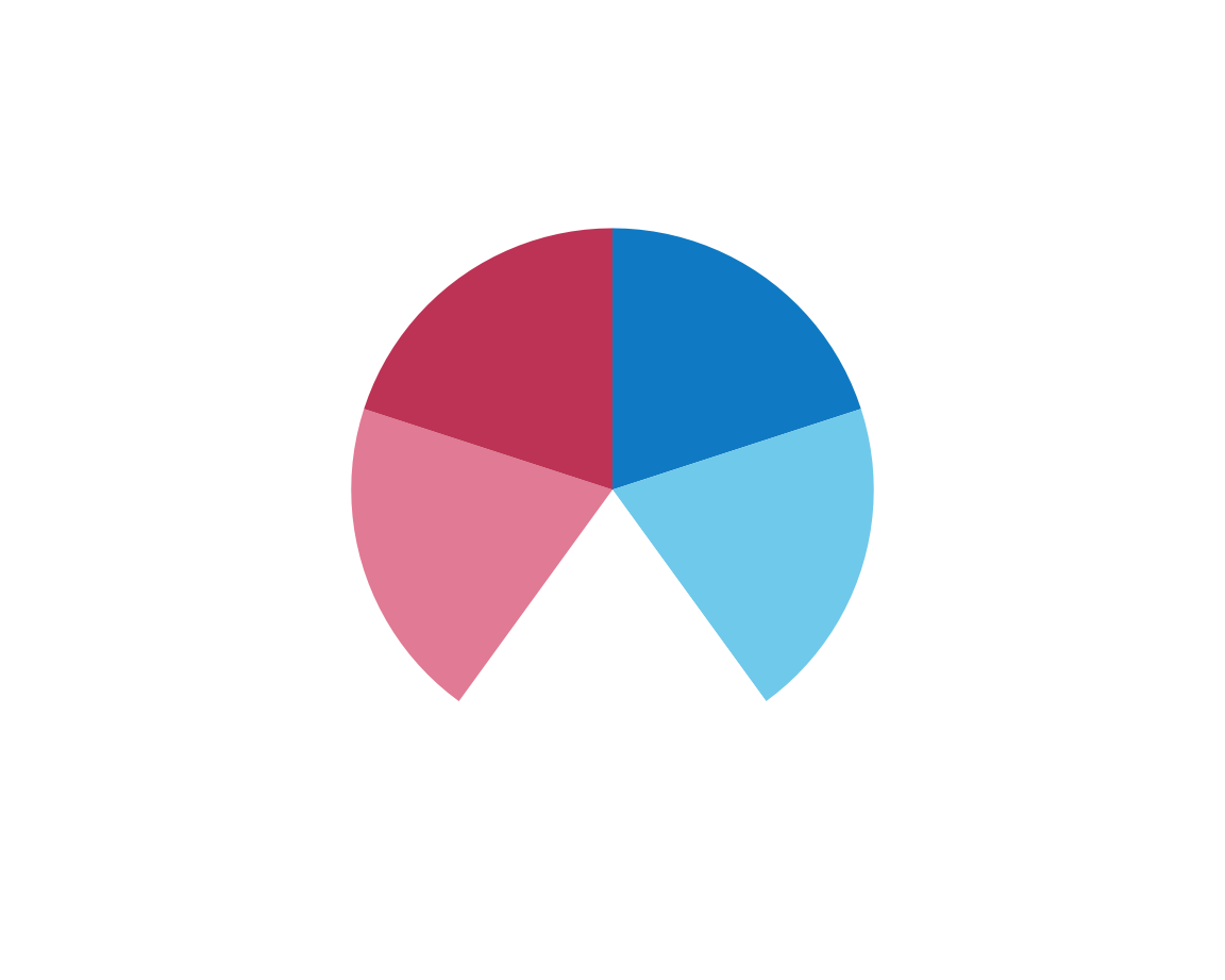
Interestingly, B seems to switch from a linear plot to a pie (or polar) plot.
To understand this better, we should check what happens when we also vary A:
plot_fn(x = 5, y = 1, A = FALSE, B = FALSE)
plot_fn(x = 5, y = 1, A = FALSE, B = TRUE)
This confirms our intuition:
Setting B = TRUE plots either a row or column of squares (depending on A) in a circular fashion (i.e., using polar coordinates).
To determine the function of the argument C does, we set it to FALSE:
plot_fn(x = 5, y = 1, A = FALSE, B = TRUE, C = FALSE)
It seems that the order of colors has changed (from regular to random). Let’s verify this for a row with 11 squares:
plot_fn(x = 11, C = TRUE)
plot_fn(x = 11, C = FALSE)
This is in line with our expectations, so we are satisfied for now. So on to argument D:
plot_fn(x = 11, D = FALSE)
plot_fn(x = 11, D = TRUE)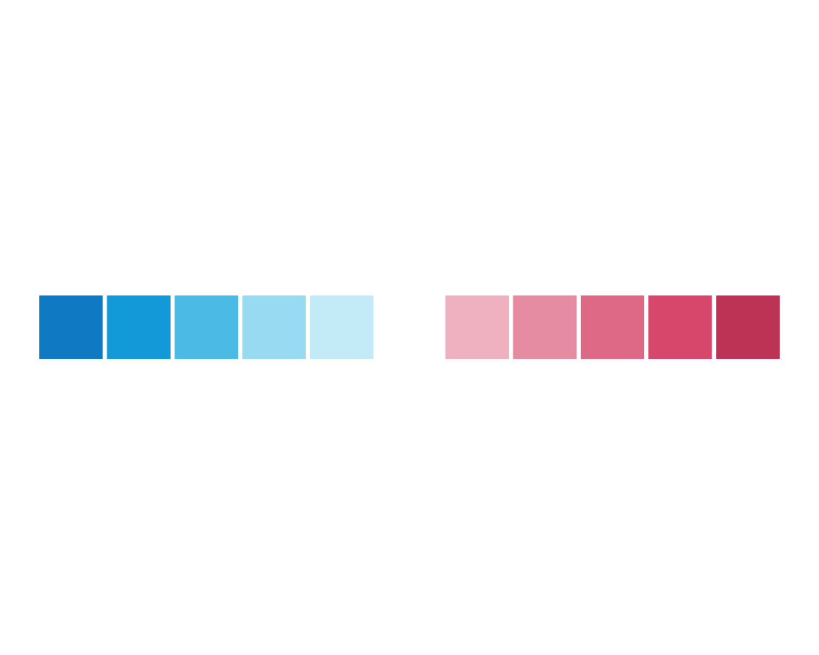
Setting D = TRUE seems to have caused some white lines to appear between the squares.
As lines have additional parameters (e.g., their width and color), we now could reconsider the argument y that we failed to understand above.
Let’s add a non-default value of y = 5 to our last command:
plot_fn(x = 11, y = 5, D = TRUE)
This supports our hypothesis that y may regulate the line width between or around squares.
As these lines are white, our attention shifts to another argument with a default of g = "white" (with a letter “g” in lowercase).
Let’s vary y and g (changing g = "white" to g = "black") to observe the effect:
plot_fn(x = 11, y = 8, D = TRUE, g = "black")
Again, our hunches are confirmed (or — for the logical positivists among us — not rejected yet). Before we decipher the meaning of the remaining arguments, let’s double check what we know so far by creating a plot with five elements that are arranged in a column and plotted in a circular fashion, with lines of width 4 in a “darkblue” color:
plot_fn(x = 5, y = 4, A = FALSE, B = TRUE, C = FALSE, D = TRUE, g = "darkblue")
Again, our intuitions are confirmed, which motivates us to tackle arguments E and F together:
plot_fn(x = 5, E = TRUE, F = FALSE)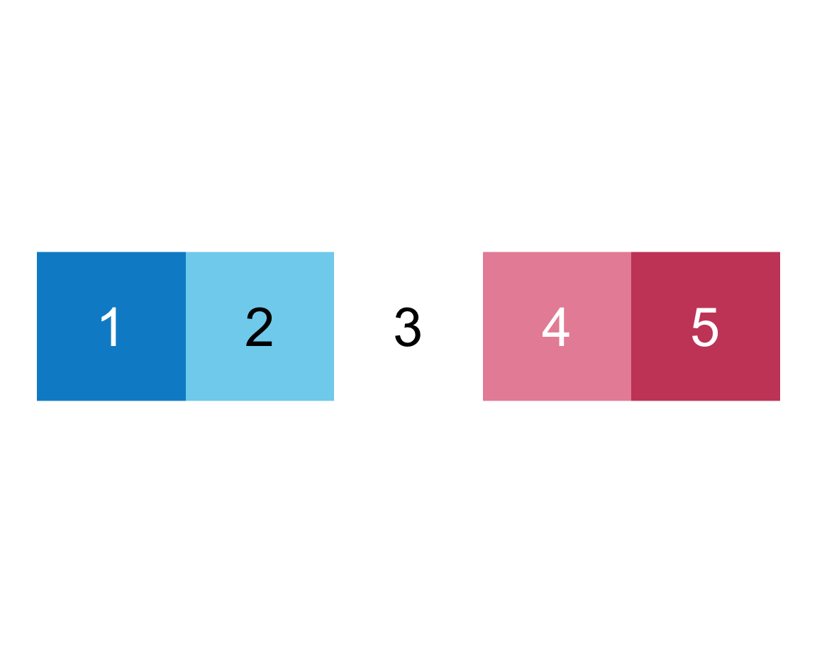
plot_fn(x = 5, E = FALSE, F = TRUE)
plot_fn(x = 5, E = TRUE, F = TRUE)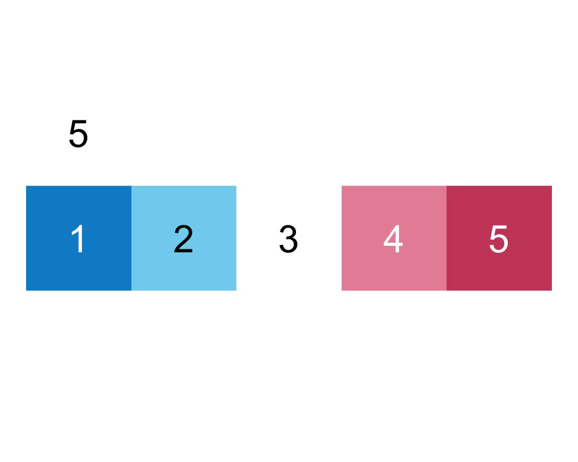
We infer that E = TRUE causes the squares to be labeled (with numbers), whereas F = TRUE adds a label above the plot (indicating the number of elements).
To see whether this also holds for other versions of the plot, we add both arguments to our more complicated command from above:
plot_fn(x = 5, y = 4, A = FALSE, B = TRUE, C = FALSE, D = TRUE, E = TRUE, F = TRUE, g = "darkblue")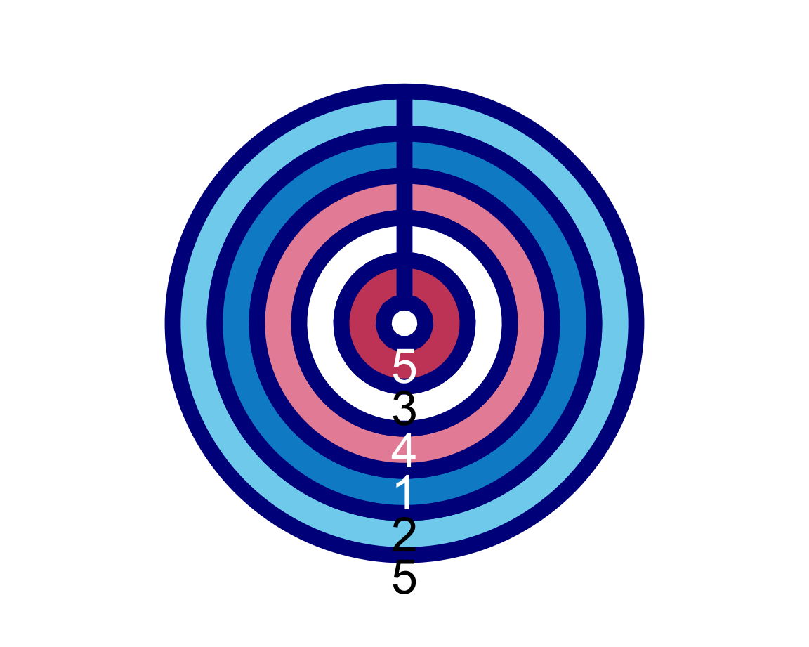
This satisfies us and leaves us only with the lowercase f as the final argument (not to be confused with uppercase F).
Its default setting of
- Default:
f = c(rev(pal_seeblau), "white", pal_pinky)
suggests that this regulates the colors of the squares or rings (using two specific color palettes of the unikn package).
To check this, we re-do our previous command with a version of f that replaces the complicated c(...) thing with a simple color “gold”:
plot_fn(x = 5, y = 4, A = FALSE, B = TRUE, C = FALSE, D = TRUE, E = TRUE, F = TRUE, g = "darkblue", f = "gold")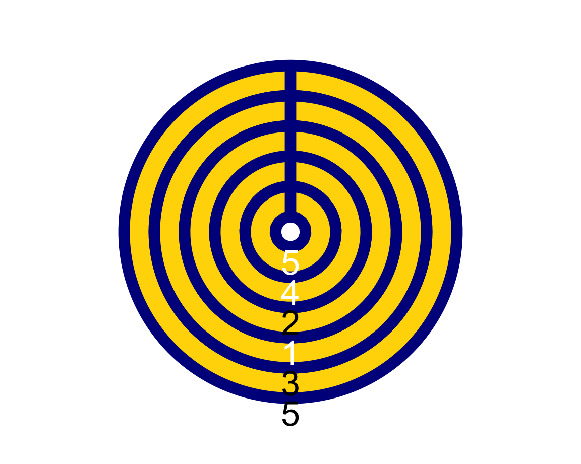
In Section 1.4, we will learn that the function c(...) defines a vector of the objects in ... (separated by commas).
To check the effect of a vector of colors on our plot, we try to set f to a vector of two color names: f = c("black", "white"),
and the line color g to "gold":
plot_fn(x = 5, y = 4, A = FALSE, B = TRUE, C = FALSE, D = TRUE, E = TRUE, F = TRUE,
        f = c("black", "white"), g = "gold")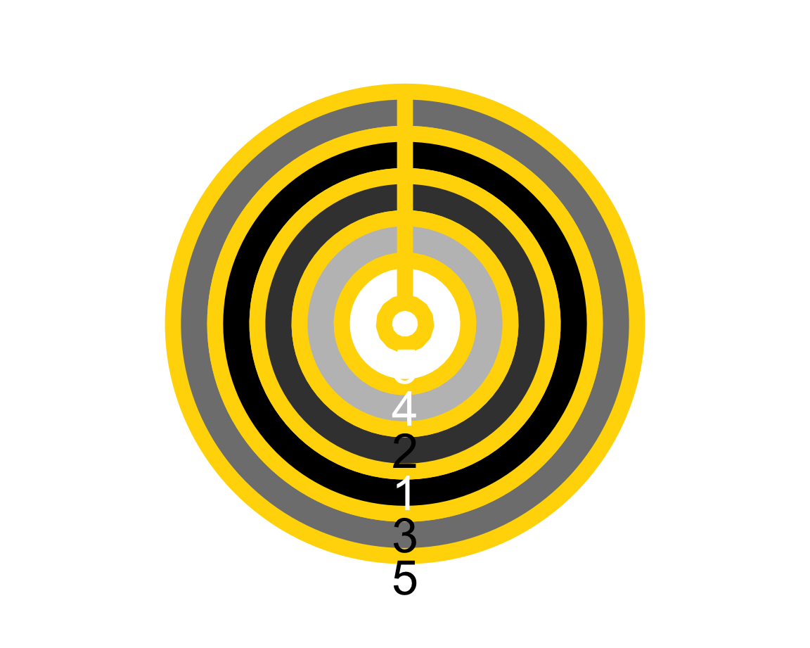
The result shows that plot_fn() uses the colors entered in f to create some color gradient (as the plot contains various shades of grey).
This concludes our exploration of plot_fn(), leaving us with the impression that this function can be used to create a wide variety of plots. Specifically, our explorations have uncovered the following meanings of the plot_fn() function’s arguments:
xA (natural) number that specifies the number of squares/segments to plot. Default:x = NA(choosing a random natural number forx).yA (decimal) number that specifies the width of lines around squares whenD = TRUE. Default:y = 1.AA Boolean value that regulates the orientation of the plot from a horizontal row (A = TRUE) to a vertical column (A = FALSE). Default:A = TRUE(i.e., row).BA Boolean value that regulates the coordinate system from linear to circular/polar. Default:B = FALSE(i.e., linear).CA Boolean value that regulates whether squares are sorted or unsorted. Default:C = TRUE(i.e., sorted).DA Boolean value that specifies whether lines should be shown around squares . Default:D = FALSE(i.e., no lines).EA Boolean value that specifies whether the squares/segments should be labeled (with numbers). Default:E = FALSE(i.e., no labels).FA Boolean value that specifies whether the plot should be labeled (with the number of parts). Default:F = FALSE(i.e., no label).fA color palette (e.g., as a vector). Default:f = c(rev(pal_seeblau), "white", pal_pinky), using color palettes from the unikn package.gA color name (e.g., as a character) for the line around squares. Default:g = "white".
Overall, our exploration has also shown that using functions is a lot easier when they have sensible names and argument names.
Practice
- We will practice exploring another complex function in Exercise 2 below (see Section 1.8.2).
As functions are our way of interacting with and manipulating data, knowing how to explore functions is a task that will accompany and enrich our entire R career. In each of the following chapters, we will explore a variety of functions written by experienced R developers, before finally learning to create our own functions (in Chapter 11).
But rather than only studying functions, we also need to learn more about key data structures in R. The following sections direct our attention on scalars (Section 1.3), vectors (Section 1.4), and rectangular tables (Section 1.5) in R.
As atomic vectors can have multiple elements, the term “atomic” refers not to their shape, but to the fact that they can only store a single data type. When only containing one element (i.e., a length of 1), an atomic vector is called a scalar.↩︎
While using
=saves typing one character, using<-distinguishes the assignment of objects from specifying arguments to functions and illustrates the direction of information flow. When writing code, being short is often a virtue. However, when misunderstandings are possible, opt for clarity, rather than brevity.↩︎More precisely, their mode is
numeric, whereas their data type isintegerordouble. However, the technical distinction of mode and type is not important here.↩︎Remember: When R is started, only the functions of base R and some other core packages are available. To use the functions or data objects provided by another package (e.g., the R package ds4psy), we first have to install the package (by calling the expression
install.packages('ds4psy')once), and then load it in our current environment (by evaluating the expressionlibrary('ds4psy')before using one of its objects).↩︎