9.5 Applications
This chapter so far has shown that working with text is challenging, but can also be rewarding and inspiring. Actually, blurring the boundaries between text and other data types is one of the most creative parts of data science. Here are some examples to sketch the scientific or artistic potential of such transgressions — and hopefully serve to stimulate your imagination.
9.5.1 Transl33ting text
So-called leet slang (aka. l33t, 1337, eleet, or leetspeak) is a system of modified spellings used primarily by online gaming or hacker communities (see the Wikipedia article leet).
The transl33t() function of ds4psy translates text into some variety of leet:
test <- "This is a simple test of leet slang."  # data

transl33t(test)
#> [1] "7h15 15 4 51mpl3 +35+ 0f l33+ 5l4ng."
paste(transl33t(letters), collapse = " ")
#> [1] "4 b c d 3 f g h 1 j k l m n 0 p q R 5 + u v w x y z"
transl33t(s)
#> [1] "7h3 c4+ 54+ 0n +h3 m4+."
#> [2] "7h3 m4d h4++3R h4d h34Rd h3R, 50 wh4+?"
#> [3] "7h3 f4+ d4d w45 50 54d."
With a little bit of practice, it actually becomes quite easy to read text in leet.
To experience this for yourself, transl33t the sentences from stringr and observe how you get faster when reading them aloud:
s3nt3nc3s <- transl33t(stringr::sentences)
tb <- tibble(#nr = 1:length(sentences),
             sentence = sentences,
             s3nt3nc3 = s3nt3nc3s)

kable(head(tb), caption = "Some sentences in l33t slang.")| sentence | s3nt3nc3 |
|---|---|
| The birch canoe slid on the smooth planks. | 7h3 b1Rch c4n03 5l1d 0n +h3 5m00+h pl4nk5. |
| Glue the sheet to the dark blue background. | Glu3 +h3 5h33+ +0 +h3 d4Rk blu3 b4ckgR0und. |
| It’s easy to tell the depth of a well. | 1+’5 345y +0 +3ll +h3 d3p+h 0f 4 w3ll. |
| These days a chicken leg is a rare dish. | 7h353 d4y5 4 ch1ck3n l3g 15 4 R4R3 d15h. |
| Rice is often served in round bowls. | R1c3 15 0f+3n 53Rv3d 1n R0und b0wl5. |
| The juice of lemons makes fine punch. | 7h3 ju1c3 0f l3m0n5 m4k35 f1n3 punch. |
The rules used by transl33t() for translating individual characters are specified in a named vector l33t_rules:
l33t_rul35
#>   a   A   e   E   i   I   o   O   s   S   T   t   r
#> "4" "4" "3" "3" "1" "1" "0" "0" "5" "5" "7" "+" "R"
By re-defining this vector, we can change the degree and the details of the conversion:
# Simpler leet rules:
my_leet <- c("e" = "3", "s" = "5", "i = 1")

transl33t(test, rules = my_leet)
#> [1] "Thi5 i5 a 5impl3 t35t of l33t 5lang."
However, with the functions for replacing characters introduced in Sections 9.3 and 9.4, we can easily design our own translations:
# (a) base R:
chartr(old = "aeistAEIST", new = "4315+4315+", x = test)

# (b) stringr:
new_leet <- c("a" = "4", "e" = "3", "i" = "1", "s" = "5", "t" = "+",
              "A" = "4", "E" = "3", "I" = "1", "S" = "5", "T" = "+")
str_replace_all(test, pattern = new_leet)
Given these skills, we are very close to creating your own transl33t() function (see Chapter 11: Functions).
We will re-visit character replacements in an exercise on naive cryptography below.
9.5.2 Detecting text in tibbles
In applied contexts, the character variable to be analyzed often does not come as an isolated vector of strings, but as a column in a larger table (or tibble). Fortunately, the commands discussed in this chapter can be used in combination with the functions discussed in the rest of this book.
For instance, we can use the stringr function str_detect() as part of a filter() command in a dplyr pipe.
As an example, the following pipe uses the tibble data_t1 from ds4psy and selects those participants whose family name (as indicated by their 2nd initial) starts with one of the letters “M,” “N,” or “O”:
df <- ds4psy::data_t1
dim(df)  # 20 cases x 4 variables
#> [1] 20  4

df %>%
  filter(str_detect(name, "[MNO].$"))
#> # A tibble: 3 × 4
#>   name  gender like_1 bnt_1
#>   <chr> <chr>   <dbl> <dbl>
#> 1 M.O.  male        4     1
#> 2 C.N.  female      4     3
#> 3 Q.N.  female      6     1
9.5.3 Counting word or character frequency
Imagine we wanted to count the number of times a word or character appears in some article or book.
As a dataset of non-trivial complexity, let’s use the 720 Harvard sentences (see Wikipedia) included in the stringr package:
# Data:
sentences <- stringr::sentences
Counting the frequency of any particular word or character is pretty straightforward with str_count():
sum(str_count(sentences, "house"))
#> [1] 7
sum(str_count(sentences, "a"))
#> [1] 1649
However, what if we wanted to know the frequencies of all possible words or characters?
To address these tasks, the ds4psy package contains two practical helpers count_words() and count_chars():
count_words(s)counts the frequency of each word ins.count_chars(s)counts the frequency of each character ins.
Both functions are case-sensitive by default (unless case_sense = FALSE) and sort their results by frequency (unless sort_freq = FALSE).
Applied to the 720 sentences, we get:
library(ds4psy)

# Frequency of words and characters:
count_words(sentences)[1:10]  # top 10 words
#> words
#> the The  of   a  to and  in  is   A was
#> 489 262 132 130 119 118  85  81  72  66
count_chars(sentences)[1:10]  # top 10 characters
#> chars
#>    e    t    a    h    o    s    r    n    i    l
#> 3054 2026 1649 1620 1552 1535 1350 1210 1191  989

# Total sums:
sum(count_words(sentences))  # number of words
#> [1] 5760
sum(count_chars(sentences))  # number of characters
#> [1] 22570
How can we solve these tasks with stringr commands discussed in Sections 9.4? And if we succeed, do we get the same results? (And if not, why not?)
Hint: These tasks can be solved by using regular expressions or by using the boundary() modifier of stringr functions.
- Counting the frequency of all words in
sentences:
# (1) counting words:
sum(str_count(sentences, regex("\\b[:alpha:]+\\b")))  # regex
#> [1] 5763
sum(str_count(sentences, boundary("word")))           # boundary modifier
#> [1] 5748

# extracing all words:
w_list <- str_extract_all(sentences, boundary("word"))
length(unlist(w_list))
#> [1] 5748
We see that the counts differ slightly, depending on the method we use. The difference between various counts can partly explained by counting vs. not counting occurrences of “s” or “t” as words:
count_words(sentences)["s"]
str_view_all(sentences, "'s", match = TRUE)

count_words(sentences)["t"]
sum(str_count(sentences, "don't"))
str_view_all(sentences, "'t", match = TRUE)- Counting the frequency of all characters in
sentences:
To address this task, we could use a fairly complicated stringr function:
# (2) counting the frequency of all characters:
all_chars <- unlist(str_extract_all(sentences, boundary("character")))
# table(all_chars)  # count frequency of all_chars

# Overall number:
length(all_chars)
#> [1] 28355
If we were only interested in the overall number of characters, there are much simpler solutions:
sum(nchar(sentences))
#> [1] 28355
sum(str_length(sentences))
#> [1] 28355
However, both these counts differ substantially from the one obtained by count_chars():
sum(count_chars(sentences))
#> [1] 22570
Again, the discrepancies between different approaches are due to different interpretations of the task.
By default, the count_chars() function removes a number of special characters (e.g., spaces, hyphens, parentheses, and punctuation characters) from the count. If these were not removed (by setting rm_specials = FALSE), we get the same overall count:
sum(count_chars(sentences, rm_specials = FALSE))
#> [1] 28355
9.5.4 Quantifying terms
Although we tried to include some meaningful examples in Sections 9.3 and 9.4, using text functions and regular expressions in real applications typically involves longer and more complicated strings of text (e.g., paragraphs, collections of articles, or books).
To illustrate a typical workflow of detecting an extracting matches, we will slightly adapt the excellent example from 14.4.2 Extract matches (Wickham & Grolemund, 2017), which detects, counts, and extracts color names in strings of text (using the sentences included in stringr). The specific tasks addressed in this example are:
- Detect, count, and obtain all
sentencesthat contain a set of common color names.
- Extract the color names contained in those sentences.
- Show the sentences containing two or more of these color names.
A key step of all these tasks is constructing a regular expression (or regex, see Appendix E) that matches any of the color names we are interested in:
# Create a regex (i.e., the pattern to search for):
colors <- c("red", "green", "blue",
            "black", "gray", "grey", "white",
            "orange", "yellow", "pink", "purple")

## Generalize example to ALL color names used in base R:
# colors <- colors()

color_match <- str_c(colors, collapse = "|")
color_match
#> [1] "red|green|blue|black|gray|grey|white|orange|yellow|pink|purple"
Equipped with this regex, we can easily detect, count, and obtain all sentences that match the pattern:
# Detect and count matching strings:
sum(str_detect(sentences, color_match))
#> [1] 69

# Obtain matching strings:
has_color <- str_subset(sentences, color_match)
length(has_color)
#> [1] 69
Thus, it appears that 69 sentences contain one of the color names in color_match.
From these sentences, we can easily extract the colors found and count (or cross-tabulate) them:
# Extract matching strings:
col_found <- str_extract(has_color, color_match)
length(col_found)  # Note: Same as length(has_color) above
#> [1] 69

# Count colors found:
table(col_found)  # base R
#> col_found
#>  black   blue   gray  green orange   pink purple    red  white yellow
#>      5      8      1      8      1      2      1     36      5      2
# tibble(col_found) %>% group_by(col_found) %>% count()  # dplyr
Note that the length of the vector col_found equals the number of sentences in has_color (i.e., both are 69).
This could either mean that every sentence found contains exactly one color name.
However, if some sentences contain more than one color name, this could also mean that the str_extract() function only extracted the first occurrence of a color from each sentence in has_color into col_found.
To find out which of these two options is the case, we can use str_count() to count the number of matches to color_match and filter sentences by the logical vector of sentences with more than one match:
# Multiple matches:
mult_match <- sentences[str_count(sentences, color_match) > 1]
str_view_all(mult_match, color_match)
Thus, some sentences contain more than one of the color names in color_match.
The fact that there exist sentences with more than one match implies that str_extract() only extracted the first match of a color from each sentence in has_color. We can double check this by counting all colors in sentences:
# Count ALL color names matched in sentences:
n_colors <- sum(str_count(sentences, color_match))
n_colors
#> [1] 74

# Note:
n_colors > length(col_found)
#> [1] TRUE
Another indication that str_extract() only extracted first matches is provided by the existence of a str_extract_all() variant of the function. As mentioned in Sections 9.4), applying this version in the context of our current tasks yields a list (here: all_col_found, rather than the 1-dimensional vector col_found above) in which some elements contain more than one color names:
# Extract ALL matching strings:
all_col_found <- str_extract_all(has_color, color_match)

# Note the difference:
is.list(all_col_found)  # a list
#> [1] TRUE
is.list(col_found)      # a vector
#> [1] FALSE
The list all_col_found can be transformed into a vector (by applying unlist() to it), which then allows counting all the matching color names found:
length(unlist(all_col_found))
#> [1] 74
table(unlist(all_col_found))
#>
#>  black   blue   gray  green orange   pink purple    red  white yellow
#>      5      8      1      8      1      2      1     40      6      2
Alternatively, setting simplify = TRUE when using str_extract_all() would return a 2-dimensional matrix in which all rows are expanded to the number of columns of the maximum number of matches:
all_col_found_mx <- str_extract_all(has_color, color_match, simplify = TRUE)

is.matrix(all_col_found_mx)
#> [1] TRUE
dim(all_col_found_mx)
#> [1] 69  2
When quantifying text for scientific purposes (e.g., for doing sentiment analysis or LSA), having the option of working with a variety of output formats is a boon, rather than a burden.
9.5.5 Plotting text
Our final example of applying string functions combines text and graphics.
Internally, the plot_text() function of ds4psy first reads in a text (from a character string x, a document file, or uses the base R function scan() to accept text input from the Console) and maps it into a table with columns for the x- and y-coordinates of each character (via the map_text_coord() function).
It then uses ggplot2 to create a tile plot of the entered text, using character frequency as a proxy for the background color of each tile (with darker colors indicating more frequent characters):
ABC_grid <- c("A B C D",
              " X Y B A",
              "A Y B X",
              " H A Z C",
              "A Z B Y",
              " D C X A")

# Plot text:
plot_text(ABC_grid)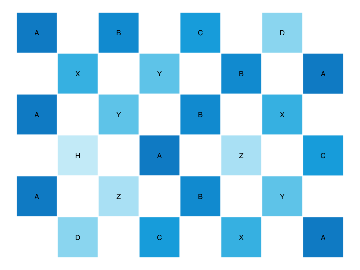
Figure 9.2: Plotting some text with plot_text().
This is not particularly creative, of course, but playing a while with plot_text() and its parameters will uncover some pleasing variations:
txt <- c("Hello world!", "This is just a test.",
         "Can you read this text?", "If so, this is good!",
         "Try using plot_text()", " for plotting text.",
         "Does this work?", "If so, this is good.",
         "Try some examples", " and then carry on...")

plot_text(txt, lbl_rotate = TRUE,
          pal = unikn::pal_bordeaux[2:5], col_lbl = "white")
Figure 9.3: Playing with plot_text() parameters.
Functions that plot text easily transcend the realm of text into the realm of visualizations. Since ordinary text already implies many graphical features (e.g., the colors, sizes, and shapes of fonts, the formatting and layout of text parts, plus many other aspects of typography), this is not new or surprising, but can still be fun.
As an example, we can use the bardr package (Billings, 2021) to load William Shakespeare’s complete works
and extract the famous Sonnet 18 (see Wikipedia):
# Get some literary work:
library(bardr)  # the complete works of William Shakespeare, as provided by Project Gutenberg

# Extract some work: Poetry > Sonnet 18
works  <- all_works_df
poetry <- subset(works, works$genre == "Poetry")
sonnet_18_start <- grep("compare thee to a summer", poetry$content)            # find 1st line
sonnet_18 <- poetry$content[(sonnet_18_start - 1):(sonnet_18_start + 14 - 1)]  # extract sonnet
sonnet_18 <- gsub(pattern = "\\\032", replacement = "'", x = sonnet_18)        # corrections
# sonnet_18

## Write text to file:
# cat(sonnet_18, file = "bard.txt", sep = "\n")- Here’s the sonnet text, as plotted by
plot_text():
plot_text(x = sonnet_18, # file = "bard.txt",
          pal = unikn::pal_seegruen[1:5],
          col_lbl = "white", cex = 2.5, borders = FALSE)
Figure 9.4: Visualizing Shakespeare’s Sonnet 18 (using the plot_text() function of ds4psy).
- Here’s a version generated by varying the color and label rotation options of
plot_chars():
# Vary colors and angles of text labels:
plot_chars(x = sonnet_18, # file = "bard.txt",
           col_lbl = c(Bordeaux, Petrol), col_bg = "white",
           cex = 2.5, fontface = 2,
           lbl_rotate = "[[:alpha:]]", angle_fg = c(-90, 90))
Figure 9.5: Varying label colors and angles in Shakespeare’s Sonnet 18 (using the plot_chars() function of ds4psy).
- If we want to locate and highlight specific target terms, we can use the regular expression options provided by the
plot_chars()function:
# Define regular expressions:
chrs_4  <- "\\b\\w{4}\\b"  # any 4-letter word
vowels  <- "[AEIOUaeiou]"  # any vowel
targets <- c("day", "nature", "summer", "winter", "spring", "fall",
             "chance", "heaven", "hell", "wind", "short", "long", "eternal",
             "live", "life", "death", "light", "shade", "time",
             month.name)
t_regex <- paste0(targets, collapse = "|")

# Locate and highlight some elements:
plot_chars(x = sonnet_18, # file = "bard.txt",
           lbl_hi = vowels, bg_hi = t_regex,
           col_lbl_hi = unikn::pal_bordeaux[3:5],
           col_bg_hi  = unikn::pal_seeblau[1],
           bg_lo = "[[:space:]|[:punct:]|[:digit:]]",
           cex = 2.5, fontface = 2)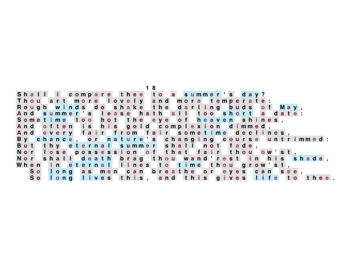
Figure 9.6: Locating and visualizing pattern matches in Shakespeare’s Sonnet 18 (using the plot_chars() function of ds4psy).
# unlink("bard.txt") # clean up text fileWhile such visualizations can be aesthetically pleasing, combining them with quantitative aspects (e.g., counting pattern matches) may also enable new insights. Overall, the boundaries between plain text and graphics are easily blurred, especially when we start thinking about word search problems, crossword puzzles, or word clouds. Thinking about new ways of visual expression will also change the ways we see characters and texts.
Practice
- Quantifying more color terms:
- Generalize the example from Section 9.5.4 to all color names that are pre-defined in base R.
Hint: The function colors() shows all 657 predefined names of colors available in base R (see Section D.3 of Appendix D).
To generalize the analysis, we only need to change the first line of code (i.e., the definition of colors):
# Create a regex (i.e., the pattern to search for):
colors <- colors()

color_match <- stringr::str_c(colors, collapse = "|")
# color_match
The regex for color_match now includes 657 color names, but all other code can be recycled from above.
- Finding and extracting
sentencescontaining common number words:
- Adopt the example from Section 9.5.4 to extracting and counting
sentencescontaining number words (i.e., the 10 count words “one,” “two,” …, “ten”).
sentences <- stringr::sentences

# Create a regex (i.e., the pattern to search for):
numbers <- c("one", "two", "three", "four", "five", "six", "seven", "eight", "nine", "ten")
n_match <- str_c(numbers, collapse = "|")
n_match
#> [1] "one|two|three|four|five|six|seven|eight|nine|ten"

# Get matching strings:
has_number <- str_subset(sentences, n_match)
length(has_number)
#> [1] 67

# Extract matching strings:
n_matches <- str_extract(has_number, n_match)
table(n_matches)
#> n_matches
#> eight  five  four   one seven   six   ten three   two
#>     2     1     1    27     2     3    20     5     6

# Multiple matches:
mult_n_match <- sentences[str_count(sentences, n_match) > 1]
str_view_all(mult_n_match, n_match)