recoding Introduction to Mediation, Moderation, and Conditional Process Analysis

10.5 When the moderator is multicategorical

10.5.1 An example.

Just as a refresher, here’s the print() output for model2.

print(model2, digits = 3)

##  Family: gaussian 
##   Links: mu = identity; sigma = identity 
## Formula: liking ~ D1 + D2 + sexism + D1:sexism + D2:sexism 
##    Data: protest (Number of observations: 129) 
## Samples: 4 chains, each with iter = 2000; warmup = 1000; thin = 1;
##          total post-warmup samples = 4000
## 
## Population-Level Effects: 
##           Estimate Est.Error l-95% CI u-95% CI Eff.Sample  Rhat
## Intercept    7.709     1.055    5.721    9.828       1502 1.001
## D1          -4.110     1.522   -7.057   -1.093       1551 1.000
## D2          -3.498     1.429   -6.246   -0.722       1415 1.001
## sexism      -0.473     0.206   -0.889   -0.077       1485 1.001
## D1:sexism    0.897     0.291    0.319    1.462       1524 1.001
## D2:sexism    0.778     0.279    0.239    1.318       1406 1.001
## 
## Family Specific Parameters: 
##       Estimate Est.Error l-95% CI u-95% CI Eff.Sample  Rhat
## sigma    1.006     0.064    0.890    1.143       2865 1.000
## 
## Samples were drawn using sampling(NUTS). For each parameter, Eff.Sample 
## is a crude measure of effective sample size, and Rhat is the potential 
## scale reduction factor on split chains (at convergence, Rhat = 1).

The Bayesian \(R^2\):

bayes_R2(model2) %>% round(digits = 3)

##    Estimate Est.Error  Q2.5 Q97.5
## R2    0.155     0.049 0.064 0.256

And the \(R^2\) difference between this and the model excluding the interaction terms:

bayes_R2(model1, summary = F) %>% 
  as_tibble() %>% 
  rename(`Model 1` = R2) %>% 
  bind_cols(
    bayes_R2(model2, summary = F) %>% 
      as_tibble() %>% 
      rename(`Model 2` = R2)
  ) %>% 
  transmute(difference = `Model 2` - `Model 1`) %>% 
  summarize(mean = mean(difference),
            ll = quantile(difference, probs = .025),
            ul = quantile(difference,  probs = .975)) %>% 
  mutate_if(is.double, round, digits = 3)

## # A tibble: 1 x 3
##    mean     ll    ul
##   <dbl>  <dbl> <dbl>
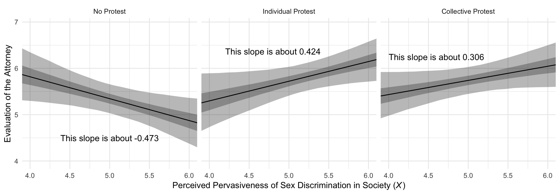
## 1 0.084 -0.039 0.202

Much like in the text, our Figure 10.7 is just a little different from what we did with Figure 10.3.

# This will help us with the `geom_text()` annotation
slopes <-
  tibble(slope = c(fixef(model2)["sexism", "Estimate"] + fixef(model2)["D1:sexism", "Estimate"],
                   fixef(model2)["sexism", "Estimate"] + fixef(model2)["D2:sexism", "Estimate"],
                   fixef(model2)["sexism", "Estimate"]),
         x = c(4.8, 4.6, 5),
         y = c(6.37, 6.25, 4.5),
         condition = c("Individual Protest", "Collective Protest", "No Protest")) %>% 
  mutate(label = str_c("This slope is about ", slope %>% round(digits = 3)),
         condition = factor(condition, levels = c("No Protest", "Individual Protest", "Collective Protest")))

# Here we plot
model2_fitted %>% 
  ggplot(aes(x = sexism)) +
  geom_ribbon(aes(ymin = Q2.5, ymax = Q97.5),
              alpha = 1/3) +
  geom_ribbon(aes(ymin = Q25, ymax = Q75),
              alpha = 1/3) +
  geom_line(aes(y = Estimate)) +
  geom_text(data = slopes,
            aes(x = x,
                y = y,
                label = label)) +
  coord_cartesian(xlim = 4:6) +
  labs(x = expression(paste("Perceived Pervasiveness of Sex Discrimination in Society (", italic(X), ")")),
       y = "Evaluation of the Attorney") +
  facet_wrap(~condition) +
  theme_minimal()

10.5.2 Probing the interaction and interpreting the regression coefficients.

We computed the posterior means for the slopes when prepping for the figure, above. Here’s how we might get more complete posterior summaries. Much like in the text, our Figure 10.7 is just a little different from what we did with Figure 10.3.

post <- 
  posterior_samples(model2) %>% 
  transmute(`No Protest` = b_sexism + `b_D1:sexism`*0 + `b_D2:sexism`*0,
            `Individual Protest` = b_sexism + `b_D1:sexism`*1 + `b_D2:sexism`*0,
            `Collective Protest` = b_sexism + `b_D1:sexism`*0 + `b_D2:sexism`*1)

post %>% 
  gather() %>% 
  mutate(key = factor(key, levels = c("No Protest", "Individual Protest", "Collective Protest"))) %>% 
  group_by(key) %>% 
  summarise(mean = mean(value),
            sd = sd(value),
            ll = quantile(value, probs = .025),
            ul = quantile(value, probs = .975)) %>% 
  mutate_if(is.double, round, digits = 3)

## # A tibble: 3 x 5
##   key                  mean    sd     ll     ul
##   <fct>               <dbl> <dbl>  <dbl>  <dbl>
## 1 No Protest         -0.473 0.206 -0.889 -0.077
## 2 Individual Protest  0.424 0.204  0.007  0.824
## 3 Collective Protest  0.306 0.182 -0.063  0.655

Here are the differences among the three protest groups.

post %>% 
  transmute(`Individual Protest - No Protest` = `Individual Protest` - `No Protest`,
            `Collective Protest - No Protest` = `Collective Protest` - `No Protest`,
            `Individual Protest - Collective Protest` = `Individual Protest` - `Collective Protest`) %>% 
  gather() %>% 
  # again, not necessary, but useful for reordering the summaries
  mutate(key = factor(key, levels = c("Individual Protest - No Protest", "Collective Protest - No Protest", "Individual Protest - Collective Protest"))) %>% 
  group_by(key) %>% 
  summarise(mean = mean(value),
            sd = sd(value),
            ll = quantile(value, probs = .025),
            ul = quantile(value, probs = .975)) %>% 
  mutate_if(is.double, round, digits = 3)

## # A tibble: 3 x 5
##   key                                      mean    sd     ll    ul
##   <fct>                                   <dbl> <dbl>  <dbl> <dbl>
## 1 Individual Protest - No Protest         0.897 0.291  0.319 1.46 
## 2 Collective Protest - No Protest         0.778 0.279  0.239 1.32 
## 3 Individual Protest - Collective Protest 0.119 0.277 -0.431 0.643