5.4 The serial multiple mediator model
5.4.1 Direct and indirect effects in a serial multiple mediator model.
5.4.2 Statistical inference.
5.4.3 Example from the presumed media influence study.
The model syntax is similar to the earlier multiple mediator model. All we change is adding import to the list of predictors in the m2_model.
m1_model <- bf(import   ~ 1 + cond)
m2_model <- bf(pmi      ~ 1 + import + cond)
y_model  <- bf(reaction ~ 1 + import + pmi + cond)
model3 <-
brm(data = pmi, family = gaussian,
y_model + m1_model + m2_model + set_rescor(FALSE),
chains = 4, cores = 4)print(model3)## Family: MV(gaussian, gaussian, gaussian)
## Links: mu = identity; sigma = identity
## mu = identity; sigma = identity
## mu = identity; sigma = identity
## Formula: reaction ~ 1 + import + pmi + cond
## import ~ 1 + cond
## pmi ~ 1 + import + cond
## Data: pmi (Number of observations: 123)
## Samples: 4 chains, each with iter = 2000; warmup = 1000; thin = 1;
## total post-warmup samples = 4000
##
## Population-Level Effects:
## Estimate Est.Error l-95% CI u-95% CI Eff.Sample Rhat
## reaction_Intercept -0.15 0.54 -1.22 0.91 4000 1.00
## import_Intercept 3.91 0.22 3.47 4.35 4000 1.00
## pmi_Intercept 4.62 0.30 4.02 5.22 4000 1.00
## reaction_import 0.32 0.07 0.18 0.47 4000 1.00
## reaction_pmi 0.40 0.09 0.21 0.58 4000 1.00
## reaction_cond 0.10 0.25 -0.39 0.60 4000 1.00
## import_cond 0.63 0.32 -0.01 1.25 4000 1.00
## pmi_import 0.20 0.07 0.06 0.33 4000 1.00
## pmi_cond 0.35 0.24 -0.11 0.82 4000 1.00
##
## Family Specific Parameters:
## Estimate Est.Error l-95% CI u-95% CI Eff.Sample Rhat
## sigma_reaction 1.31 0.09 1.15 1.49 4000 1.00
## sigma_import 1.73 0.11 1.53 1.98 4000 1.00
## sigma_pmi 1.28 0.08 1.13 1.46 4000 1.00
##
## Samples were drawn using sampling(NUTS). For each parameter, Eff.Sample
## is a crude measure of effective sample size, and Rhat is the potential
## scale reduction factor on split chains (at convergence, Rhat = 1).The \(R^2\) posterior densities:
bayes_R2(model3, summary = F) %>%
  as_tibble() %>%
  gather() %>%
  mutate(key = str_remove(key, "R2_")) %>%

  ggplot(aes(x = value, color = key, fill = key)) +
  geom_density(alpha = .5) +
  scale_color_ptol() +
  scale_fill_ptol() +
  scale_y_continuous(NULL, breaks = NULL) +
  coord_cartesian(xlim = 0:1) +
  labs(title = expression(paste("The ", italic("R")^{2}, " distributions for model3, the serial multiple mediator model")),
       subtitle = "The density for reaction hasn't changed from model2. However, look how the pmi density separated from import.",
       x = NULL) +
  theme_minimal() +
  theme(legend.title = element_blank())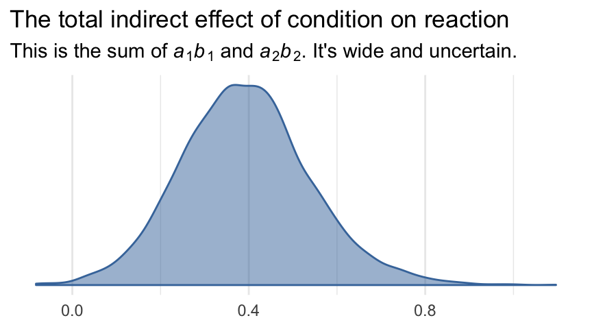
As before, here we’ll save the posterior samples into a data frame and rename the parameters a bit to match Hayes’s nomenclature.
post <- posterior_samples(model3)

post <-
  post %>%
  mutate(a1 = b_import_cond,
         a2 = b_pmi_cond,
         b1 = b_reaction_import,
         b2 = b_reaction_pmi,
         c_prime = b_reaction_cond,
         d21 = b_pmi_import)
Here are the parameter summaries for the pathways depicted in Figure 5.6.
post %>%
  select(a1:d21) %>%
  gather() %>%
  group_by(key) %>%
  summarize(mean = mean(value),
            median = median(value),
            ll = quantile(value, probs = .025),
            ul = quantile(value, probs = .975)) %>%
  mutate_if(is_double, round, digits = 3)
## # A tibble: 6 x 5
## key mean median ll ul
## <chr> <dbl> <dbl> <dbl> <dbl>
## 1 a1 0.628 0.632 -0.007 1.25
## 2 a2 0.349 0.345 -0.111 0.825
## 3 b1 0.325 0.324 0.183 0.466
## 4 b2 0.396 0.397 0.206 0.577
## 5 c_prime 0.105 0.108 -0.388 0.602
## 6 d21 0.196 0.196 0.064 0.326To get our version of the parameter summaries in Table 5.2, all you have to do is add the summaries for the intercepts to what we did above.
post %>%
  rename(im1 = b_import_Intercept,
         im2 = b_pmi_Intercept,
         iy = b_reaction_Intercept) %>%
  select(a1:d21, starts_with("i")) %>%
  gather() %>%
  group_by(key) %>%
  summarize(mean = mean(value),
            median = median(value),
            ll = quantile(value, probs = .025),
            ul = quantile(value, probs = .975)) %>%
  mutate_if(is_double, round, digits = 3)
## # A tibble: 9 x 5
## key mean median ll ul
## <chr> <dbl> <dbl> <dbl> <dbl>
## 1 a1 0.628 0.632 -0.007 1.25
## 2 a2 0.349 0.345 -0.111 0.825
## 3 b1 0.325 0.324 0.183 0.466
## 4 b2 0.396 0.397 0.206 0.577
## 5 c_prime 0.105 0.108 -0.388 0.602
## 6 d21 0.196 0.196 0.064 0.326
## 7 im1 3.91 3.91 3.47 4.35
## 8 im2 4.62 4.61 4.02 5.22
## 9 iy -0.151 -0.163 -1.22 0.913Here we compute the four indirect effects.
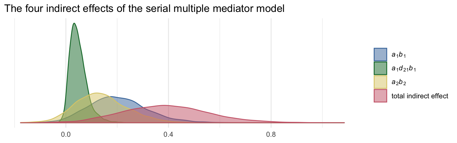
post <-
  post %>%
  mutate(a1b1 = a1*b1,
         a2b2 = a2*b2,
         a1d21b2 = a1*d21*b2) %>%
  mutate(total_indirect_effect = a1b1 + a2b2 + a1d21b2)
The summaries for the indirect effects are as follows.
post %>%
  select(a1b1:total_indirect_effect) %>%
  gather() %>%
  group_by(key) %>%
  summarize(mean = mean(value),
            median = median(value),
            ll = quantile(value, probs = .025),
            ul = quantile(value, probs = .975)) %>%
  mutate_if(is_double, round, digits = 3)
## # A tibble: 4 x 5
## key mean median ll ul
## <chr> <dbl> <dbl> <dbl> <dbl>
## 1 a1b1 0.203 0.196 -0.002 0.449
## 2 a1d21b2 0.049 0.043 -0.001 0.131
## 3 a2b2 0.139 0.132 -0.043 0.357
## 4 total_indirect_effect 0.39 0.386 0.08 0.743To get the contrasts Hayes presented in page 179, we just do a little subtraction.
post %>%
  transmute(C1 = a1b1 - a2b2,
            C2 = a1b1 - a1d21b2,
            C3 = a2b2 - a1d21b2) %>%
  gather() %>%
  group_by(key) %>%
  summarize(mean = mean(value),
            median = median(value),
            ll = quantile(value, probs = .025),
            ul = quantile(value, probs = .975)) %>%
  mutate_if(is_double, round, digits = 3)
## # A tibble: 3 x 5
## key mean median ll ul
## <chr> <dbl> <dbl> <dbl> <dbl>
## 1 C1 0.064 0.065 -0.244 0.386
## 2 C2 0.154 0.145 -0.004 0.374
## 3 C3 0.09 0.086 -0.11 0.311And just because it’s fun, we may as well plot our indirect effects.
# this will help us save a little space with the plot code
my_labels <- c(expression(paste(italic(a)[1], italic(b)[1])),
               expression(paste(italic(a)[1], italic(d)[21], italic(b)[1])),
               expression(paste(italic(a)[2], italic(b)[2])),
               "total indirect effect")
post %>%
  select(a1b1:total_indirect_effect) %>%
  gather() %>%

  ggplot(aes(x = value, fill = key, color = key)) +
  geom_density(alpha = .5) +
  scale_color_ptol(NULL, labels = my_labels,
                   guide = guide_legend(label.hjust = 0)) +
  scale_fill_ptol(NULL, labels = my_labels,
                   guide = guide_legend(label.hjust = 0)) +
  scale_y_continuous(NULL, breaks = NULL) +
  labs(title = "The four indirect effects of the serial multiple mediator model",
       x = NULL) +
  theme_minimal()