13.5 Relative conditional direct effects
In order to get the \(R^2\) difference distribution analogous to the change in \(R^2\) \(F\)-test Hayes discussed on pages 495–496, we’ll have to first refit the model without the interaction for the \(Y\) criterion, liking.
m_model <- bf(respappr ~ 1 + D1 + D2 + sexism + D1:sexism + D2:sexism)
y_model <- bf(liking   ~ 1 + D1 + D2 + respappr + sexism)

model3 <-
  brm(data = protest, family = gaussian,
      m_model + y_model + set_rescor(FALSE),
      chains = 4, cores = 4)
Here’s the \(\Delta R^2\) density.
R2s <-
  bayes_R2(model1, resp = "liking", summary = F) %>%
  as_tibble() %>%
  rename(model1 = R2_liking) %>%
  bind_cols(
    bayes_R2(model3, resp = "liking", summary = F) %>%
      as_tibble() %>%
      rename(model3 = R2_liking)
  ) %>%
  mutate(difference = model1 - model3)

R2s %>%
  ggplot(aes(x = difference, y = 0)) +

  geom_halfeyeh(point_interval = median_qi, .prob = c(0.95, 0.5),
                fill = "grey50", color = "white") +
  scale_x_continuous(breaks = c(-.5, median(R2s$difference) %>% round(2), .5)) +
  scale_y_continuous(NULL, breaks = NULL) +
  coord_cartesian(xlim = c(-.5, .5)) +
  xlab(expression(paste(Delta, italic(R)^2))) +
  theme_black() +
  theme(panel.grid = element_blank())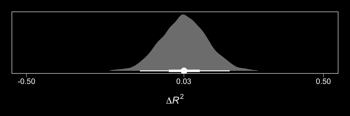
We’ll also compare the models by their information criteria.
loo(model1, model3)## LOOIC SE
## model1 760.10 29.56
## model3 761.61 31.10
## model1 - model3 -1.51 5.47waic(model1, model3)## WAIC SE
## model1 759.74 29.47
## model3 761.39 31.05
## model1 - model3 -1.65 5.46As when we went through these steps for resp = "respappr", above, the Bayesian \(R^2\), the LOO-CV, and the WAIC all suggest there’s little difference between the two models with respect to predictive utility. In such a case, I’d lean on theory to choose between them. If inclined, one could also do Bayesian model averaging.
Our approach to plotting the relative conditional direct effects will mirror what we did for the relative conditional indirect effects, above. Here are the brm() parameters that correspond to the parameter names of Hayes’s notation.
- \(c_{1}\) =
b_liking_D1 - \(c_{2}\) =
b_liking_D2 - \(c_{4}\) =
b_liking_D1:sexism - \(c_{5}\) =
b_liking_D2:sexism
With all clear, we’re off to the races.
# c1 + c4W
D1_function <- function(w){
  post$b_liking_D1 + post$`b_liking_D1:sexism`*w
  }

# c2 + c5W
D2_function <- function(w){
  post$b_liking_D2 + post$`b_liking_D2:sexism`*w
  }

rcde_tibble <-
  tibble(sexism = seq(from = 3.5, to = 6.5, length.out = 30)) %>%
  group_by(sexism) %>%
  mutate(`Protest vs. No Protest`            = map(sexism, D1_function),
         `Collective vs. Individual Protest` = map(sexism, D2_function)) %>%
  unnest() %>%
  ungroup() %>%
  mutate(iter = rep(1:4000, times = 30)) %>%
  gather(`direct effect`, value, -sexism, -iter) %>%
  mutate(`direct effect` = factor(`direct effect`, levels = c("Protest vs. No Protest", "Collective vs. Individual Protest")))

head(rcde_tibble)
## # A tibble: 6 x 4
## sexism iter `direct effect` value
## <dbl> <int> <fct> <dbl>
## 1 3.5 1 Protest vs. No Protest -0.856
## 2 3.5 2 Protest vs. No Protest -0.482
## 3 3.5 3 Protest vs. No Protest -1.24
## 4 3.5 4 Protest vs. No Protest -1.23
## 5 3.5 5 Protest vs. No Protest -1.06
## 6 3.5 6 Protest vs. No Protest -0.663Here is our variant of Figure 13.4, with respect to the relative conditional direct effects.
rcde_tibble %>%
  group_by(`direct effect`, sexism) %>%
  summarize(median = median(value),
            ll = quantile(value, probs = .025),
            ul = quantile(value, probs = .975)) %>%

  ggplot(aes(x = sexism, group = `direct effect`)) +
  geom_ribbon(aes(ymin = ll, ymax = ul),
              color = "white", fill = "transparent", linetype = 3) +
  geom_line(aes(y = median),
            color = "white") +
  coord_cartesian(xlim = 4:6,
                  ylim = c(-.6, .8)) +
  labs(x = expression(paste("Perceived Pervasiveness of Sex Discrimination in Society (", italic(W), ")")),
       y = "Relative Conditional Effect on Liking") +
  theme_black() +
  theme(panel.grid = element_blank(),
        legend.position = "none") +
  facet_grid(~ `direct effect`)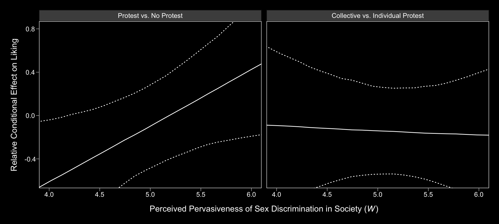
Holy smokes, them are some wide 95% CIs! No wonder the information criteria and \(R^2\) comparisons were so uninspiring.
Notice that the y-axis is on the parameter space. In Hayes’s Figure 13.5, the y-axis is on the liking space, instead. When we want things in the parameter space, we work with the output of posterior_samples(); when we want them in the criterion space, we use fitted().
# we need new `nd` data
nd <-
  tibble(D1 = rep(c(1/3, -2/3, 1/3), each = 30),
         D2 = rep(c(1/2, 0, -1/2), each = 30),
         respappr = mean(protest$respappr),
         sexism = seq(from = 3.5, to = 6.5, length.out = 30) %>% rep(., times = 3))

# we feed `nd` into `fitted()`
model1_fitted <-
  fitted(model1,
       newdata = nd,
       resp = "liking",
       summary = T) %>%
  as_tibble() %>%
  bind_cols(nd) %>%
  mutate(condition = ifelse(D2 == 0, "No Protest",
                            ifelse(D2 == -1/2, "Individual Protest", "Collective Protest"))) %>%
  mutate(condition = factor(condition, levels = c("No Protest", "Individual Protest", "Collective Protest")))

model1_fitted %>%
  ggplot(aes(x = sexism, group = condition)) +
  geom_ribbon(aes(ymin = Q2.5, ymax = Q97.5),
              linetype = 3, color = "white", fill = "transparent") +
  geom_line(aes(y = Estimate), color = "white") +
  geom_point(data = protest, aes(x = sexism, y = liking),
             color = "red", size = 2/3) +
  coord_cartesian(xlim = 4:6,
                  ylim = 4:7) +
  labs(x = expression(paste("Perceived Pervasiveness of Sex Discrimination in Society (", italic(W), ")")),
       y = expression(paste("Evaluation of the Attorney (", italic(Y), ")"))) +
  theme_black() +
  theme(panel.grid = element_blank()) +
  facet_wrap(~condition)
We expanded the range of the y-axis, a bit, to show more of that data (and there’s even more data outside of our expanded range). Also note how after doing so and after including the 95% CI bands, the crossing regression line effect in Hayes’s Figure 13.5 isn’t as impressive looking any more.
On pages 497–498, Hayes discussed more omnibus \(F\)-tests. Much like with the \(M\) criterion, we won’t come up with Bayesian \(F\)-tests, but we might go ahead and make pairwise comparisons at the three percentiles Hayes prefers.
# we need new `nd` data
nd <-
  tibble(D1 = rep(c(1/3, -2/3, 1/3), each = 3),
         D2 = rep(c(1/2, 0, -1/2), each = 3),
         respappr = mean(protest$respappr),
         sexism = rep(c(4.250, 5.120, 5.896), times = 3))

# this tie we'll use `summary = F`
model1_fitted <-
  fitted(model1,
       newdata = nd,
       resp = "liking",
       summary = F) %>%
  as_tibble() %>%
  gather() %>%
  mutate(condition = rep(c("Collective Protest", "No Protest", "Individual Protest"),
                         each = 3*4000),
         sexism = rep(c(4.250, 5.120, 5.896), times = 3) %>% rep(., each = 4000),
         iter = rep(1:4000, times = 9)) %>%
  select(-key) %>%
  spread(key = condition, value = value) %>%
  mutate(`Individual Protest - No Protest` = `Individual Protest` - `No Protest`,
         `Collective Protest - No Protest` = `Collective Protest` - `No Protest`,
         `Collective Protest - Individual Protest` = `Collective Protest` - `Individual Protest`)

# a tiny bit more wrangling and we're ready to plot the difference distributions
model1_fitted %>%
  select(sexism, contains("-")) %>%
  gather(key, value, -sexism) %>%

  ggplot(aes(x = value)) +
  geom_halfeyeh(aes(y = 0), fill = "grey50", color = "white",
                point_interval = median_qi, .prob = 0.95) +
  geom_vline(xintercept = 0, color = "grey25", linetype = 2) +
  scale_y_continuous(NULL, breaks = NULL) +
  facet_grid(sexism~key) +
  theme_black() +
  theme(panel.grid = element_blank())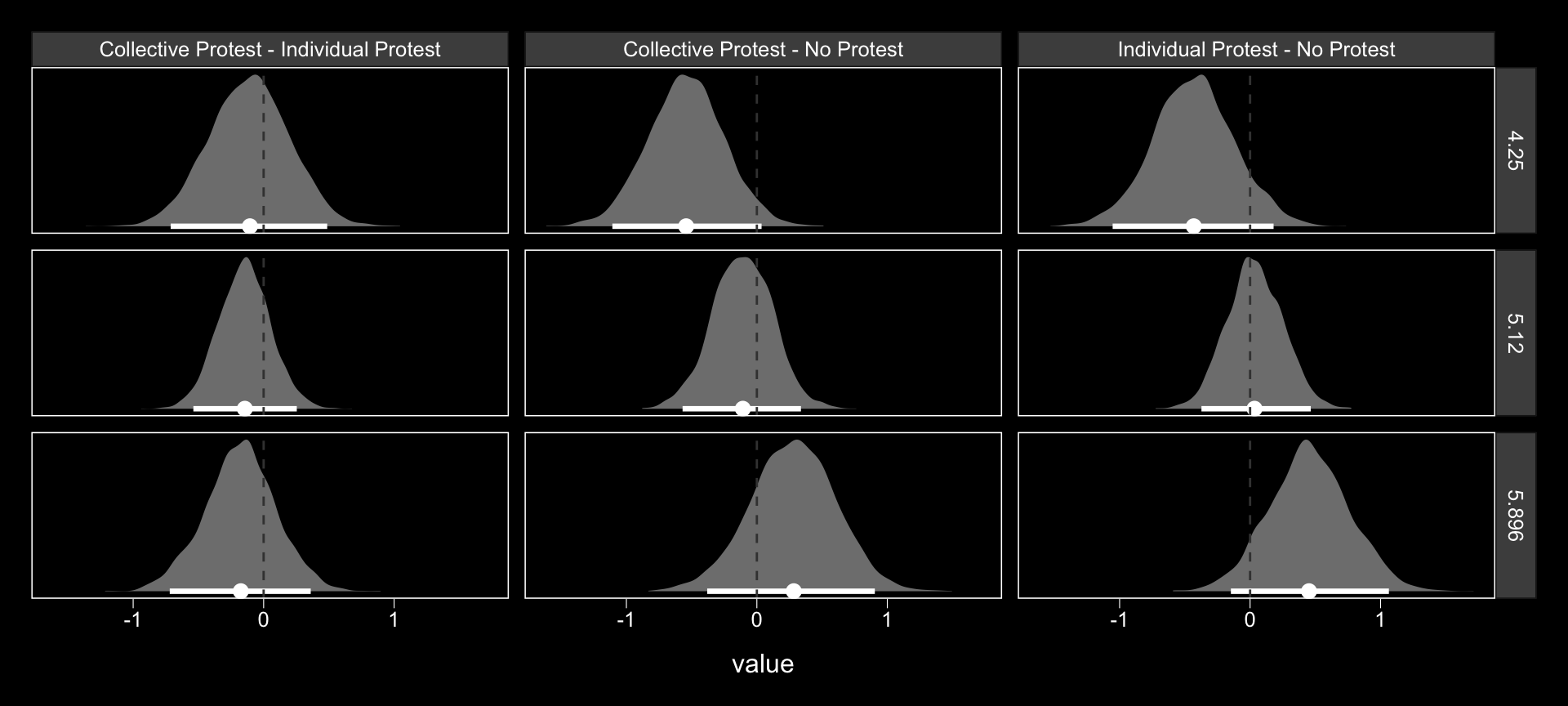
Now we have model1_fitted, it’s easy to get the typical numeric summaries for the differences.
model1_fitted %>%
  select(sexism, contains("-")) %>%
  gather(key, value, -sexism) %>%
  group_by(key, sexism) %>%
  summarize(mean = mean(value),
            ll = quantile(value, probs = .025),
            ul = quantile(value, probs = .975)) %>%
  mutate_if(is.double, round, digits = 3)
## # A tibble: 9 x 5
## # Groups: key [3]
## key sexism mean ll ul
## <chr> <dbl> <dbl> <dbl> <dbl>
## 1 Collective Protest - Individual Protest 4.25 -0.11 -0.713 0.487
## 2 Collective Protest - Individual Protest 5.12 -0.147 -0.539 0.254
## 3 Collective Protest - Individual Protest 5.90 -0.179 -0.72 0.361
## 4 Collective Protest - No Protest 4.25 -0.542 -1.11 0.036
## 5 Collective Protest - No Protest 5.12 -0.109 -0.569 0.338
## 6 Collective Protest - No Protest 5.90 0.277 -0.381 0.904
## 7 Individual Protest - No Protest 4.25 -0.432 -1.05 0.18
## 8 Individual Protest - No Protest 5.12 0.038 -0.373 0.465
## 9 Individual Protest - No Protest 5.90 0.456 -0.147 1.06We don’t have \(p\)-values, but all the differences are small in magnitude and have wide 95% intervals straddling zero.
To get the difference scores Hayes presented on pages 498–500, one might:
post %>%
  mutate(`Difference in liking between being told she protested or not when W is 4.250` = b_liking_D1 + `b_liking_D1:sexism`*4.250,
         `Difference in liking between being told she protested or not when W is 5.120` = b_liking_D1 + `b_liking_D1:sexism`*5.120,
         `Difference in liking between being told she protested or not when W is 5.896` = b_liking_D1 + `b_liking_D1:sexism`*5.896,

         `Difference in liking between collective vs. individual protest when W is 4.250` = b_liking_D2 + `b_liking_D2:sexism`*4.250,
         `Difference in liking between collective vs. individual protest when W is 5.120` = b_liking_D2 + `b_liking_D2:sexism`*5.120,
         `Difference in liking between collective vs. individual protest when W is 5.896` = b_liking_D2 + `b_liking_D2:sexism`*5.896) %>%
  select(contains("Difference in liking")) %>%
  gather() %>%
  group_by(key) %>%
  summarize(mean = mean(value),
            ll = quantile(value, probs = .025),
            ul = quantile(value, probs = .975)) %>%
  mutate_if(is.double, round, digits = 3)
## # A tibble: 6 x 4
## key mean ll ul
## <chr> <dbl> <dbl> <dbl>
## 1 Difference in liking between being told she protested or not when W is 4.250 -0.487 -1.00 0.017
## 2 Difference in liking between being told she protested or not when W is 5.120 -0.036 -0.43 0.35
## 3 Difference in liking between being told she protested or not when W is 5.896 0.367 -0.207 0.923
## 4 Difference in liking between collective vs. individual protest when W is 4.2… -0.11 -0.713 0.487
## 5 Difference in liking between collective vs. individual protest when W is 5.1… -0.147 -0.539 0.254
## 6 Difference in liking between collective vs. individual protest when W is 5.8… -0.179 -0.72 0.361