2.2 The simple linear regression model
Here is how one might get the simple OLS coefficients in base R with the lm() function.
(model2 <- lm(data = glbwarm, govact ~ 1 + negemot))
#>
#> Call:
#> lm(formula = govact ~ 1 + negemot, data = glbwarm)
#>
#> Coefficients:
#> (Intercept)      negemot
#>       2.757        0.514
For more detailed output, put the model object model2 into the summary() function.
summary(model2)
#>
#> Call:
#> lm(formula = govact ~ 1 + negemot, data = glbwarm)
#>
#> Residuals:
#>    Min     1Q Median     3Q    Max
#> -4.329 -0.673  0.102  0.755  3.214
#>
#> Coefficients:
#>             Estimate Std. Error t value Pr(>|t|)
#> (Intercept)   2.7573     0.0987    27.9   <2e-16 ***
#> negemot       0.5142     0.0255    20.2   <2e-16 ***
#> ---
#> Signif. codes:  0 '***' 0.001 '**' 0.01 '*' 0.05 '.' 0.1 ' ' 1
#>
#> Residual standard error: 1.11 on 813 degrees of freedom
#> Multiple R-squared:  0.334,  Adjusted R-squared:  0.333
#> F-statistic:  407 on 1 and 813 DF,  p-value: <2e-16
Here’s the Bayesian model in brms.
model2 <-
  brm(data = glbwarm, family = gaussian,
      govact ~ 1 + negemot,
      chains = 4, cores = 4)
There are several ways to get a brms model summary. A go-to is with the print() function.
print(model2)
#>  Family: gaussian
#>   Links: mu = identity; sigma = identity
#> Formula: govact ~ 1 + negemot
#>    Data: glbwarm (Number of observations: 815)
#> Samples: 4 chains, each with iter = 2000; warmup = 1000; thin = 1;
#>          total post-warmup samples = 4000
#>
#> Population-Level Effects:
#>           Estimate Est.Error l-95% CI u-95% CI Eff.Sample Rhat
#> Intercept     2.76      0.10     2.56     2.96       4000 1.00
#> negemot       0.51      0.03     0.46     0.57       3803 1.00
#>
#> Family Specific Parameters:
#>       Estimate Est.Error l-95% CI u-95% CI Eff.Sample Rhat
#> sigma     1.11      0.03     1.06     1.17       4000 1.00
#>
#> Samples were drawn using sampling(NUTS). For each parameter, Eff.Sample
#> is a crude measure of effective sample size, and Rhat is the potential
#> scale reduction factor on split chains (at convergence, Rhat = 1).
The summary() function works very much the same way. To get a more focused look, you can use the posterior_summary() function:
posterior_summary(model2)
#>              Estimate Est.Error      Q2.5     Q97.5
#> b_Intercept     2.758    0.1021     2.556     2.956
#> b_negemot       0.514    0.0261     0.462     0.565
#> sigma           1.112    0.0275     1.060     1.167
#> lp__        -1248.621    1.2617 -1251.883 -1247.216
That also yields the log posterior, lp__, which you can learn more about here or here. We won’t focus on the lp__ directly in this project.
But anyways, the Q2.5 and Q97.5, are the lower- and upper-levels of the 95% credible intervals. The Q prefix stands for quantile (see this thread). In this case, these are a renamed version of the l-95% CI and u-95% CI columns from our print() output.
To make a quick plot of the regression line, one can use the convenient marginal_effects() function.
marginal_effects(model2)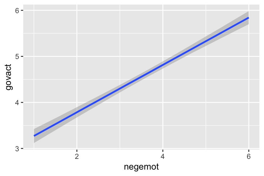
If you want to customize that output, you might nest it in plot().
plot(marginal_effects(model2),
     points = T,
     point_args = c(height = .05, width = .05,
                    alpha = 1/2, size = 1/3))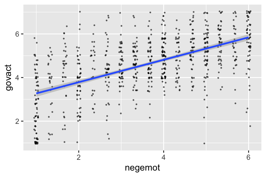
It’s also useful to be able to work with the output of a brms model directly. For our first step, we’ll put our HMC draws into a data frame.
post <- posterior_samples(model2)

head(post)
#>   b_Intercept b_negemot sigma  lp__
#> 1        2.73     0.525  1.05 -1250
#> 2        2.86     0.505  1.11 -1249
#> 3        2.76     0.520  1.11 -1247
#> 4        2.98     0.446  1.12 -1251
#> 5        2.91     0.462  1.08 -1250
#> 6        2.77     0.512  1.12 -1247
Next, we’ll use the fitted() function to simulate model-implied summaries for the expected govact value, given particular predictor values. Our first model only has negemot as a predictor, and we’ll ask for the expected govact values for negemot ranging from 0 to 7.
nd <- tibble(negemot = seq(from = 0, to = 7, length.out = 30))

f_model2 <-
  fitted(model2,
         newdata = nd) %>%
  as_tibble() %>%
  bind_cols(nd)

f_model2
#> # A tibble: 30 x 5
#>   Estimate Est.Error  Q2.5 Q97.5 negemot
#>      <dbl>     <dbl> <dbl> <dbl>   <dbl>
#> 1     2.76    0.102   2.56  2.96   0
#> 2     2.88    0.0963  2.69  3.07   0.241
#> 3     3.01    0.0906  2.83  3.18   0.483
#> 4     3.13    0.0849  2.96  3.29   0.724
#> 5     3.25    0.0794  3.10  3.41   0.966
#> 6     3.38    0.0739  3.23  3.52   1.21
#> # ... with 24 more rows
The first two columns should look familiar to the output from print(model2), above. The next two columns, Q2.5 and Q97.5, are the lower- and upper-levels of the 95% credible intervals, like we got from posterior_samples(). We got the final column with the bind_cols(nd) code.
Here’s our bespoke version of Figure 2.4.
glbwarm %>%
  group_by(negemot, govact) %>%
  count() %>%

  ggplot(aes(x = negemot)) +
  geom_point(aes(y = govact, size = n)) +
  geom_ribbon(data = f_model2,
              aes(ymin = Q2.5,
                  ymax = Q97.5),
              fill = "grey75", alpha = 3/4) +
  geom_line(data = f_model2,
            aes(y = Estimate)) +
  annotate("text", x = 2.2, y = 7.5, label = "Cases with positive residuals", color = "red3") +
  annotate("text", x = 4.75, y = .8, label = "Cases with negative residuals", color = "blue3") +
  labs(x = expression(paste("NEGEMOT: Negative emotions about climate change (", italic("X"), ")")),
       y = expression(paste("GOVACT: Support for governmentaction (", italic("Y"), ")"))) +
  coord_cartesian(xlim = range(glbwarm$negemot)) +
  theme_bw() +
  theme(legend.position = "none")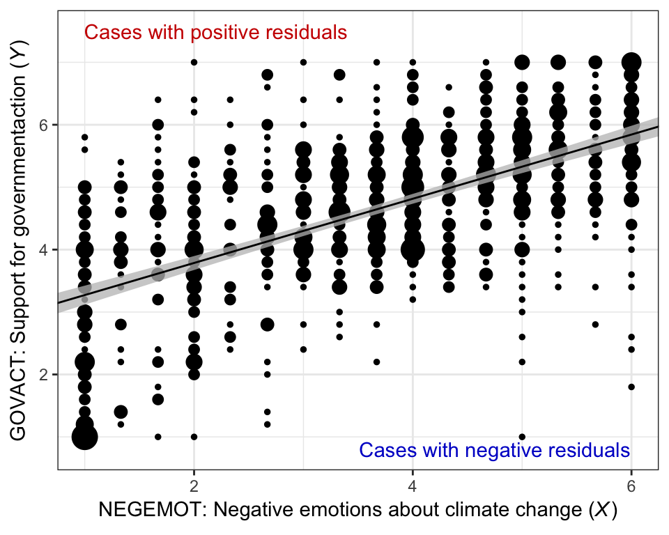
2.2.1 Interpretation of the constant and regression coefficient
Nothing to recode, here.
2.2.2 The standardized regression model
Same here.
2.2.3 Simple linear regression with a dichotomous antecedent variable.
Here we add sex to the model.
model3 <-
  brm(data = glbwarm, family = gaussian,
      govact ~ 1 + sex,
chains = 4, cores = 4)print(model3)
#> Family: gaussian
#> Links: mu = identity; sigma = identity
#> Formula: govact ~ 1 + sex
#> Data: glbwarm (Number of observations: 815)
#> Samples: 4 chains, each with iter = 2000; warmup = 1000; thin = 1;
#> total post-warmup samples = 4000
#>
#> Population-Level Effects:
#> Estimate Est.Error l-95% CI u-95% CI Eff.Sample Rhat
#> Intercept 4.72 0.07 4.58 4.85 3872 1.00
#> sex -0.27 0.10 -0.45 -0.07 3960 1.00
#>
#> Family Specific Parameters:
#> Estimate Est.Error l-95% CI u-95% CI Eff.Sample Rhat
#> sigma 1.36 0.03 1.29 1.42 4000 1.00
#>
#> Samples were drawn using sampling(NUTS). For each parameter, Eff.Sample
#> is a crude measure of effective sample size, and Rhat is the potential
#> scale reduction factor on split chains (at convergence, Rhat = 1).Our model output is very close to that in the text. If you just wanted the coefficients, you might use the fixef() function.
fixef(model3) %>% round(digits = 3)
#>           Estimate Est.Error  Q2.5  Q97.5
#> Intercept    4.716     0.068  4.58  4.850
#> sex         -0.265     0.097 -0.45 -0.073
Though not necessary, we used the round() function to reduce the number of significant digits in the output.
You can get a little more information with the posterior_summary() function.
But since Bayesian estimation yields an entire posterior distribution, you can visualize that distribution in any number of ways. Because we’ll be using ggplot2, we’ll need to put the posterior draws into a data frame before plotting.
post <- posterior_samples(model3)We could summarize the posterior with boxplots:
post %>%
  rename(female = b_Intercept) %>%
  mutate(male = female + b_sex) %>%
  select(male, female) %>%
  gather() %>%

  ggplot(aes(x = key, y = value)) +
  geom_boxplot(aes(fill = key)) +
  theme_bw() +
  theme(legend.position = "none")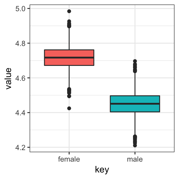
Or with overlapping density plots:
post %>%
  rename(female = b_Intercept) %>%
  mutate(male = female + b_sex) %>%
  select(male, female) %>%
  gather() %>%

  ggplot(aes(x = value, group = key, fill = key)) +
  geom_density(color = "transparent", alpha = 3/4) +
  theme_bw()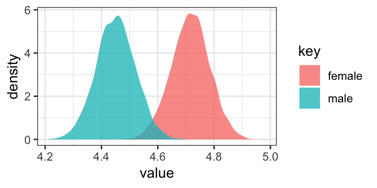
Or even with violin plots with superimposed posterior medians and 95% intervals:
post %>%
  rename(female = b_Intercept) %>%
  mutate(male = female + b_sex) %>%
  select(male, female) %>%
  gather() %>%

  ggplot(aes(x = key, y = value)) +
  geom_violin(aes(fill = key), color = "transparent", alpha = 3/4) +
  stat_summary(fun.y = median,
               fun.ymin = function(i){quantile(i, probs = .025)},
               fun.ymax = function(i){quantile(i, probs = .975)}) +
  theme_bw() +
  theme(legend.position = "none")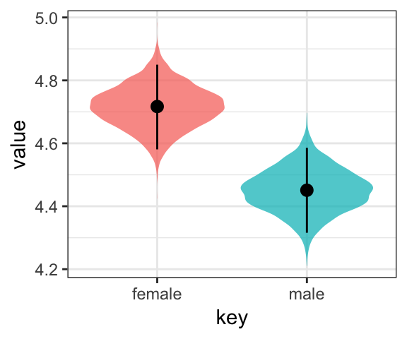
For even more ideas, see Matthew Kay’s tidybayes package. You can also get a sense of the model estimates for women and men with a little addition. Here we continue to use the round() function to simplify the output.
# for women
round(fixef(model3)[1, ], digits = 2)
#>  Estimate Est.Error      Q2.5     Q97.5
#>      4.72      0.07      4.58      4.85

# for men
round(fixef(model3)[1, ] + fixef(model3)[2, ], digits = 2)
#>  Estimate Est.Error      Q2.5     Q97.5
#>      4.45      0.17      4.13      4.78
Here’s the partially-standardized model, first with lm().
glbwarm <-
  glbwarm %>%
  mutate(govact_z = (govact - mean(govact))/sd(govact))

lm(data = glbwarm, govact_z ~ 1 + sex)
#>
#> Call:
#> lm(formula = govact_z ~ 1 + sex, data = glbwarm)
#>
#> Coefficients:
#> (Intercept)          sex
#>      0.0963      -0.1972
Now we’ll use Bayes.
model3_p_z <-
  brm(data = glbwarm, family = gaussian,
      govact_z ~ 1 + sex,
chains = 4, cores = 4)fixef(model3_p_z)
#> Estimate Est.Error Q2.5 Q97.5
#> Intercept 0.0979 0.0477 0.00333 0.1916
#> sex -0.1996 0.0688 -0.33517 -0.0664