3.3 Statistical inference
3.3.1 Inference about the total effect of \(X\) on \(Y\).
3.3.2 Inference about the direct effect of \(X\) on \(Y\).
In this section, Hayes provided a \(t\)-test and corresponding \(p\)-value for the direct effect (i.e., \(c'\), b_reaction_cond). Instead of the \(t\)-test, we can just look at the posterior distribution.
post %>%

  ggplot(aes(x = b_reaction_cond)) +
  geom_density(color = "transparent",
               fill = colorblind_pal()(4)[4]) +
  geom_vline(xintercept = 0, color = "white", linetype = 2) +
  scale_y_continuous(NULL, breaks = NULL) +
  labs(title = expression(paste("Yep, 0 is a credible value for ", italic("c"), ".")),
       x = NULL) +
  theme_classic()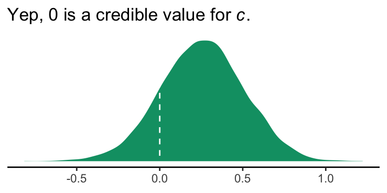
If you wanted to quantify what proportion of the density was less than 0, you could do:
post %>%
  summarize(proportion_below_zero = filter(., b_reaction_cond < 0) %>% nrow()/nrow(.))
## proportion_below_zero
## 1 0.1505This is something like a Bayesian \(p\)-value. But of course, you could always just look at the posterior intervals.
posterior_interval(model1)["b_reaction_cond", ]## 2.5% 97.5%
## -0.2432898 0.74764493.3.3 Inference about the indirect of \(X\) on \(Y\) through \(M\).
3.3.3.1 The normal theory approach.
This is not our approach.
3.3.3.2 Bootstrap confidence interval.
This is not our approach.
However, Markov chain Monte Carlo (MCMC) methods are iterative and share some characteristics with boostrapping. On page 98, Hayes outlined 6 steps for constructing the \(ab\) bootstrap confidence interval. Here are our responses to those steps w/r/t Bayes with MCMC–or in our case HMC (i.e., Hamiltonian Monte Carlo).
If HMC or MCMC, in general, are new to you, you might check out this lecture or the Stan reference manual if you’re more technically oriented.
Anyway, Hayes’s 6 steps:
3.3.3.2.1 Step 1.
With HMC we do not take random samples of the data themselves. Rather, we take random draws from the posterior distribution. The posterior distribution is the joint probability distribution of our model.
3.3.3.2.2 Step 2.
After we fit our model with the brm() function and save our posterior draws in a data frame (i.e., post <- posterior_samples(my_model_fit)), we then make a new column (a.k.a. vector, variable) that is the product of our coefficients for the \(a\) and \(b\) pathways. In the example above, this looked like post %>% mutate(ab = b_pmi_cond*b_reaction_pmi). Let’s take a look at those columns.
post %>%
  select(b_pmi_cond, b_reaction_pmi, ab) %>%
  slice(1:10)
## b_pmi_cond b_reaction_pmi ab
## 1 0.4105134 0.2303314 0.09455412
## 2 0.3417169 0.7141880 0.24405010
## 3 0.7714622 0.2955409 0.22799862
## 4 0.5577318 0.5939846 0.33128411
## 5 0.4799405 0.4863486 0.23341837
## 6 0.8622422 0.6712376 0.57876937
## 7 0.3388167 0.5585035 0.18923030
## 8 0.6320108 0.5958088 0.37655762
## 9 0.2710269 0.6620422 0.17943122
## 10 0.2677347 0.6401424 0.17138832Our data frame, post, has 4000 rows. Why 4000? By default, brms runs 4 HMC chains. Each chain has 2000 iterations, 1000 of which are warmups, which we always discard. As such, there are 1000 good iterations left in each chain and \(1000\times4 = 4000\). We can change these defaults as needed.
Each row in post contains the parameter values based on one of those draws. And again, these are draws from the posterior distribution. They are not draws from the data.
3.3.3.2.3 Step 3.
We don’t refit the model \(k\) times based on the samples from the data. We take a number of draws from the posterior distribution. Hayes likes to take 5000 samples when he bootstraps. Happily, that number is quite similar to our 4000 HMC draws. Whether 5000, 4000 or 10,000, these are all large enough numbers that the distributions become fairly stable. With HMC, however, you might want to increase the number of iterations if the effective sample size, ‘Eff.Sample’ in the print() output, is substantially smaller than the number of iterations.
3.3.3.2.4 Step 4.
When we use the quantile() function to compute our Bayesian credible intervals, we’ve sorted. Conceptually, we’ve done this:
post %>%
  select(ab) %>%
  arrange(ab) %>%
  slice(1:10)
## ab
## 1 -0.19874481
## 2 -0.17442439
## 3 -0.15657977
## 4 -0.15650372
## 5 -0.13878656
## 6 -0.12153300
## 7 -0.10987695
## 8 -0.10746942
## 9 -0.10168737
## 10 -0.097588383.3.3.2.5 Step 5.
Yes, this is what we do, too.
ci <- 95

.5*(100 - ci)
## [1] 2.53.3.3.2.6 Step 6.
This is also what we do.
ci <- 95

(100 - .5*(100 - ci))
## [1] 97.5Also, notice the headers in the rightmost two columns in our posterior_summary() output:
posterior_summary(model1)## Estimate Est.Error Q2.5 Q97.5
## b_reaction_Intercept 0.5328574 0.55479853 -5.576345e-01 1.6452479
## b_pmi_Intercept 5.3779538 0.16817860 5.056328e+00 5.6954178
## b_reaction_pmi 0.5044945 0.09774672 3.093958e-01 0.6968369
## b_reaction_cond 0.2566901 0.25232357 -2.432898e-01 0.7476449
## b_pmi_cond 0.4744565 0.24039142 -5.044517e-03 0.9364379
## sigma_reaction 1.4093572 0.09208966 1.241056e+00 1.6010297
## sigma_pmi 1.3195622 0.08718468 1.164042e+00 1.5044898
## lp__ -434.8809615 1.97212737 -4.397098e+02 -432.1698836Those .025 and .975 quantiles from above are just what brms is giving us in our 95% Bayesian credible intervals.
Here’s our version of Figure 3.5.
# these will come in handy in the subtitle
ll <- quantile(post$ab, probs = .025) %>% round(digits = 3)
ul <- quantile(post$ab, probs = .975) %>% round(digits = 3)

post %>%

  ggplot(aes(x = ab)) +
  geom_histogram(color = "white", size = .25,
               fill = colorblind_pal()(5)[5],
               binwidth = .025, boundary = 0) +
  geom_vline(xintercept = quantile(post$ab, probs = c(.025, .975)),
             linetype = 3, color = colorblind_pal()(6)[6]) +
  labs(x = expression(paste("Indirect effect (", italic("ab"), ")")),
       y = "Frequency in 4,000 HMC posterior draws",
       subtitle = paste("95% of the posterior draws are between", ll, "and", ul)) +
  theme_classic()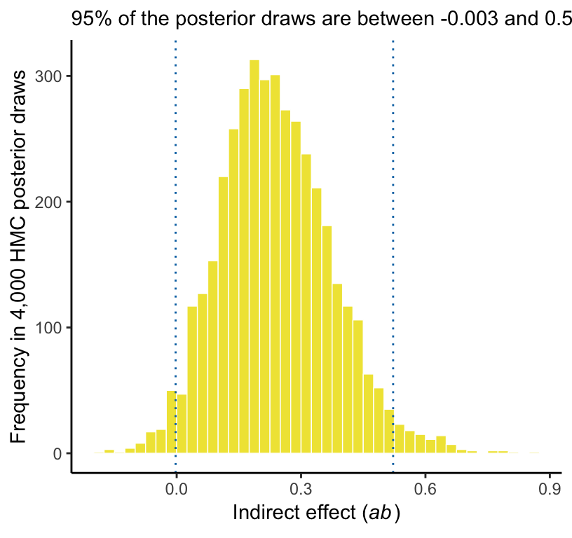
Again, as Hayes discussed how to specify different types of intervals in PROCESS on page 102, you can ask for different kinds of intervals in your print() or summary() output with the probs argument, just as you can with quantile() when working directly with the posterior draws.
Hayes discussed setting the seed in PROCESS on page 104. You can do this with the seed argument in the brm() function, too.
3.3.3.3 Alternative “asymmetric” confidence interval approaches.
This section does not quite refer to us. I’m a little surprised Hayes didn’t at least dedicate a paragraph or two on Bayesian estimation. Sure, he mentioned Monte Carlo, but not within the context of Bayes. So it goes…