2.6 Statistical inference
Here’s a tidyverse way to do Hayes’s simulation. We’re just using OLS regression with the lm() function. You could do this with Bayesian HMC estimation, but man would it take a while. For our first step, we’ll define two custom functions.
# this first one will use the `sample_n()` function to randomly sample from `glbwarm`
make_sample <- function(i){
  set.seed(i)
  sample_n(glbwarm, 50, replace = F)
}

# this second function will fit our model, the same one from `model4`, to each of our subsamples
glbwarm_model <- function(df) {
  lm(govact ~ 1 + negemot + posemot + ideology + sex + age, data = df)
}
Now we’ll run the simulation, wrangle the output, and plot in one fell swoop.
# we need an iteration index, which will double as the values we set our seed with in our `make_sample()` function
tibble(iter = 1:1e4) %>%
  group_by(iter) %>%
  # inserting our subsamples
  mutate(sample = map(iter, make_sample)) %>%
  # fitting our models
  mutate(model = map(sample, glbwarm_model)) %>%
  # taking those model results and tidying them with the broom package
  mutate(broom = map(model, broom::tidy)) %>%
  # unnesting allows us to access our model results
  unnest(broom) %>%
  # we're only going to focus on the estimates for `negemot`
  filter(term == "negemot") %>%

  # Here it is, Figure 2.7
  ggplot(aes(x = estimate)) +
  geom_histogram(binwidth = .025, boundary = 0) +
  labs(x = "Unstandardized regression coefficient for negemot",
       y = "Frequency in 1e4 samples of size 50") +
  theme_bw()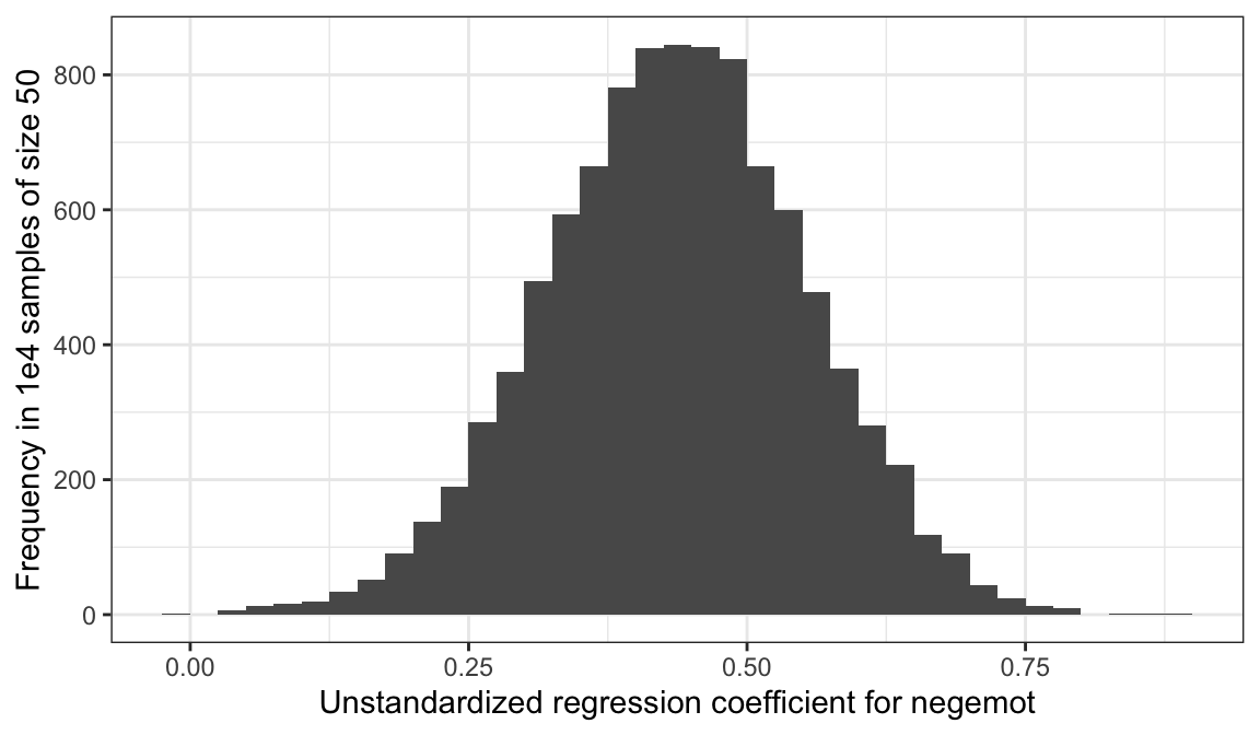
To learn more about this approach to simulations, see this section of R4DS.
2.6.1 Testing a null hypothesis.
As Bayesians, we don’t need to wed ourselves to the null hypothesis. We’re not interested in the probability of the data given the null hypothesis. Bayes’s rule,
\[p(\theta|D) = \frac{p(D|\theta)p(\theta)}{p(D)}\]
gives us the probability of the model parameters, given the data. Though I acknowledge different researchers might set out to ask different things of their data, I propose we’re generally more interested in determining the most probable parameter values than we are the probabilities tested within the NHST paradigm.
posterior_samples(model4) %>%

  ggplot(aes(x = b_negemot)) +
  geom_density(fill = "black", color = "transparent") +
  geom_vline(xintercept = posterior_interval(model4)["b_negemot", ],
             color = "white", linetype = 2) +
  scale_x_continuous(breaks = posterior_interval(model4)["b_negemot", ] %>% as.double(),
                     labels = posterior_interval(model4)["b_negemot", ] %>% as.double() %>% round(digits = 2) %>% as.character()) +
  scale_y_continuous(NULL, breaks = NULL) +
  labs(subtitle = "The most probable values for our b_negemot parameter are the ones around the peak\nof the density. For convenience, the dashed lines denote the 95% credible intervals.\nSure, you could ask yourself, 'Is zero within those intervals?' But with such rich output,\nthat seems like an impoverished question to ask.") +
  theme_bw()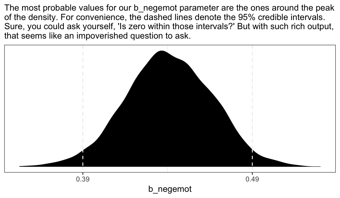
2.6.2 Interval estimation.
Within the Bayesian paradigm, we don’t use 95% intervals based on the typical frequentist formula. With the brms package, we typically use percentile-based intervals. Take the 95% credible intervals for the negemot coefficient from model model4:
posterior_interval(model4)["b_negemot", ]
#>  2.5% 97.5%
#> 0.389 0.491
We can actually get those intervals with the simple use of the base R quantile() function.
posterior_samples(model4) %>%
  summarize(the_2.5_percentile = quantile(b_negemot, probs = .025),
            the_97.5_percentile = quantile(b_negemot, probs = .975))
#>   the_2.5_percentile the_97.5_percentile
#> 1              0.389               0.491
The consequence of this is that our Bayesian credible intervals aren’t necessarily symmetric. Which is fine because the posterior distribution for a given parameter isn’t always symmetric.
But not all Bayesian intervals are percentile based. John Kruschke, for example, often recommends highest posterior density intervals in his work. The brms package doesn’t have a convenience function for these, but you can compute them with help from the HDInterval package.
library(HDInterval)

hdi(posterior_samples(model4)[ , "b_negemot"], credMass = .95)
#> lower upper
#> 0.388 0.488
#> attr(,"credMass")
#> [1] 0.95
Finally, because Bayesians aren’t bound to the NHST paradigm, we aren’t bound to 95% intervals, either. For example, in both his excellent text and as a default in its accompanying rethinking package, Richard McElreath often uses 89% intervals. Alternatively, Andrew Gelman has publically advocated for 50% intervals. The most important thing is to express the uncertainty in the posterior in a clearly-specified way. If you’d like, say, 80% intervals in your model summary, you can insert a prob argument into either print() or summary().
print(model4, prob = .8)
#>  Family: gaussian
#>   Links: mu = identity; sigma = identity
#> Formula: govact ~ 1 + negemot + posemot + ideology + sex + age
#>    Data: glbwarm (Number of observations: 815)
#> Samples: 4 chains, each with iter = 2000; warmup = 1000; thin = 1;
#>          total post-warmup samples = 4000
#>
#> Population-Level Effects:
#>           Estimate Est.Error l-80% CI u-80% CI Eff.Sample Rhat
#> Intercept     4.06      0.20     3.80     4.31       4000 1.00
#> negemot       0.44      0.03     0.41     0.47       4000 1.00
#> posemot      -0.03      0.03    -0.06     0.01       4000 1.00
#> ideology     -0.22      0.03    -0.25    -0.18       4000 1.00
#> sex          -0.01      0.08    -0.11     0.09       4000 1.00
#> age          -0.00      0.00    -0.00     0.00       4000 1.00
#>
#> Family Specific Parameters:
#>       Estimate Est.Error l-80% CI u-80% CI Eff.Sample Rhat
#> sigma     1.07      0.03     1.04     1.10       4000 1.00
#>
#> Samples were drawn using sampling(NUTS). For each parameter, Eff.Sample
#> is a crude measure of effective sample size, and Rhat is the potential
#> scale reduction factor on split chains (at convergence, Rhat = 1).
Note how two of our columns changed to ‘l-80% CI’ and ‘u-80% CI’.
You can specify custom percentile levels with posterior_summary():
posterior_summary(model4, probs = c(.9, .8, .7, .6, .4, .3, .2, .1)) %>%
  round(digits = 2)
#>             Estimate Est.Error      Q90      Q80      Q70      Q60      Q40      Q30      Q20      Q10
#> b_Intercept     4.06      0.20     4.31     4.23     4.17     4.11     4.01     3.96     3.89     3.80
#> b_negemot       0.44      0.03     0.47     0.46     0.45     0.45     0.43     0.43     0.42     0.41
#> b_posemot      -0.03      0.03     0.01     0.00    -0.01    -0.02    -0.03    -0.04    -0.05    -0.06
#> b_ideology     -0.22      0.03    -0.18    -0.20    -0.20    -0.21    -0.22    -0.23    -0.24    -0.25
#> b_sex          -0.01      0.08     0.09     0.05     0.03     0.01    -0.03    -0.05    -0.08    -0.11
#> b_age           0.00      0.00     0.00     0.00     0.00     0.00     0.00     0.00     0.00     0.00
#> sigma           1.07      0.03     1.10     1.09     1.08     1.07     1.06     1.06     1.05     1.04
#> lp__        -1215.77      1.83 -1213.73 -1214.24 -1214.63 -1215.03 -1215.93 -1216.45 -1217.15 -1218.26
And of course, you can use multiple interval summaries when you summarize() the output from posterior_samples(). E.g.,
posterior_samples(model4) %>%
  select(b_Intercept:b_age) %>%
  gather() %>%
  group_by(key) %>%
  summarize(`l-95% CI` = quantile(value, probs = .025),
            `u-95% CI` = quantile(value, probs = .975),
            `l-50% CI` = quantile(value, probs = .25),
            `u-50% CI` = quantile(value, probs = .75)) %>%
  mutate_if(is.double, round, digits = 2)
#> # A tibble: 6 x 5
#>   key         `l-95% CI` `u-95% CI` `l-50% CI` `u-50% CI`
#>   <chr>            <dbl>      <dbl>      <dbl>      <dbl>
#> 1 b_age            -0.01       0          0          0
#> 2 b_ideology       -0.27      -0.16      -0.24      -0.2
#> 3 b_Intercept       3.66       4.45       3.92       4.2
#> 4 b_negemot         0.39       0.49       0.42       0.46
#> 5 b_posemot        -0.08       0.03      -0.05      -0.01
#> 6 b_sex            -0.16       0.14      -0.06       0.04
Throughout this project, I’m going to be lazy and default to conventional 95% intervals, with occasional appearances of 50% intervals.
2.6.3 Testing a hypothesis about a set of antecedent variables.
Here we’ll make use of the update() function to hastily fit our reduced model, model5.
model5 <-
  update(model4,
         govact ~ 1 + ideology + sex + age,
         chains = 4, cores = 4)
We can get a look at the \(R^2\) summaries for our competing models like this.
bayes_R2(model4) %>% round(digits = 2)
#>    Estimate Est.Error Q2.5 Q97.5
#> R2     0.39      0.02 0.35  0.43
bayes_R2(model5) %>% round(digits = 2)
#>    Estimate Est.Error Q2.5 Q97.5
#> R2     0.18      0.02 0.14  0.22
So far, it looks like our fuller model, model4, explains more variation in the data. If we wanted to look at their distributions, we’d set summary = F in the bayes_R2() function and convert the results to a data frame or tibble. Here we use bind_cols() to put the \(R^2\) results for both in the same tibble.
R2s <-
  bayes_R2(model4, summary = F) %>%
  as_tibble() %>%
  rename(R2_model4 = R2) %>%
  bind_cols(
    bayes_R2(model5, summary = F) %>%
      as_tibble() %>%
      rename(R2_model5 = R2)
  )

head(R2s)
#> # A tibble: 6 x 2
#>   R2_model4 R2_model5
#>       <dbl>     <dbl>
#> 1     0.374     0.177
#> 2     0.402     0.239
#> 3     0.383     0.174
#> 4     0.397     0.181
#> 5     0.372     0.178
#> 6     0.404     0.184
With our R2s tibble in hand, we’re ready to plot.
R2s %>%
  gather() %>%

  ggplot(aes(x = value, fill = key)) +
  geom_density(color = "transparent") +
  scale_y_continuous(NULL, breaks = NULL) +
  coord_cartesian(xlim = 0:1) +
  theme_bw()
Yep, the \(R^2\) distribution for model4, the one including the emotion variables, is clearly larger than that for the more parsimonious model5. And it’d just take a little more data wrangling to get a formal \(R^2\) difference score.
R2s %>%
  mutate(difference = R2_model5 - R2_model4) %>%

  ggplot(aes(x = difference)) +
  geom_density(fill = "black", color = "transparent") +
  scale_y_continuous(NULL, breaks = NULL) +
  coord_cartesian(xlim = -1:0) +
  labs(title = expression(paste(Delta, italic("R")^{2})),
       subtitle = expression(paste("This is the amount the ", italic("R")^{2}, " dropped after pruning the emotion variables from the model.")),
       x = NULL) +
  theme_bw()
The \(R^2\) approach is popular within the social sciences. But it has its limitations, the first of which is that it doesn’t correct for model complexity. The second is it’s not applicable to a range of models, such as those that do not use the Gaussian likelihood (e.g., logistic regression) or to multilevel models.
Happily, information criteria offer a more general framework. The AIC is the most popular information criteria among frequentists. Within the Bayesian world, we have the DIC, the WAIC, and the LOO. The DIC is quickly falling out of favor and is not immediately available with the brms package. However, we can use the WAIC and the LOO, both of which are computed in brms via the loo package.
In brms, you can get the WAIC or LOO values with waic() or loo(), respectively. Here we use loo() and save the output as objects.
l_model4 <- loo(model4)
l_model5 <- loo(model5)
Here’s the main loo-summary output for model4.
l_model4
#>
#> Computed from 4000 by 815 log-likelihood matrix
#>
#>          Estimate   SE
#> elpd_loo  -1213.7 22.7
#> p_loo         7.5  0.6
#> looic      2427.5 45.5
#> ------
#> Monte Carlo SE of elpd_loo is 0.0.
#>
#> All Pareto k estimates are good (k < 0.5).
#> See help('pareto-k-diagnostic') for details.
You get a wealth of output, more of which can be seen with str(l_model4). For now, notice the “All pareto k estimates are good (k < 0.5).” Pareto \(k\) values can be used for diagnostics. Each case in the data gets its own \(k\) value and we like it when those \(k\)s are low. The makers of the loo package get worried when those \(k\)s exceed 0.7 and as a result, loo() spits out a warning message when they do. Happily, we have no such warning messages in this example.
If you want to work with the \(k\) values directly, you can extract them and place them into a tibble like so:
l_model4$diagnostics %>%
  as_tibble()
#> # A tibble: 815 x 2
#>   pareto_k n_eff
#>      <dbl> <dbl>
#> 1  -0.120  3973.
#> 2  -0.143  3992.
#> 3   0.0169 3890.
#> 4   0.311  2405.
#> 5  -0.0462 3997.
#> 6  -0.126  3966.
#> # ... with 809 more rows
The pareto_k values can be used to examine cases that are overly-influential on the model parameters, something akin to a Cook’s \(D_{i}\). See, for example this discussion on stackoverflow.com in which several members of the Stan team weighed in. The issue is also discussed in this paper and in this lecture by Aki Vehtari.
But anyway, we’re getting ahead of ourselves. Back to the LOO.
Like other information criteria, the LOO values aren’t of interest in and of themselves. However, the values of one model’s LOO relative to that of another is of great interest. We generally prefer models with lower information criteria. With compare_ic(), we can compute a formal difference score between multiple loo objects.
compare_ic(l_model4, l_model5)
#>                 LOOIC   SE
#> model4           2427 45.5
#> model5           2666 41.1
#> model4 - model5  -238 31.8
We also get a standard error. Here it looks like model4 was substantially better, in terms of LOO-values, than model5.
For more on the LOO, see the loo reference manual, this handy vignette, or the scholarly papers referenced therein. Also, although McElreath doesn’t discuss the LOO, he does cover the topic in general in his text and in his online lectures on the topic.