recoding Introduction to Mediation, Moderation, and Conditional Process Analysis

2.1 Correlation and prediction

Here we load a couple necessary packages, load the data, and take a peek.

library(tidyverse)

glbwarm <- read_csv("data/glbwarm/glbwarm.csv")

glimpse(glbwarm)
#> Observations: 815
#> Variables: 7
#> $ govact   <dbl> 3.6, 5.0, 6.6, 1.0, 4.0, 7.0, 6.8, 5.6, 6.0, 2.6, 1.4, 5.6, 7.0, 3.8, 3.4, 4.2, 1.0, 2.6...
#> $ posemot  <dbl> 3.67, 2.00, 2.33, 5.00, 2.33, 1.00, 2.33, 4.00, 5.00, 5.00, 1.00, 4.00, 1.00, 5.67, 3.00...
#> $ negemot  <dbl> 4.67, 2.33, 3.67, 5.00, 1.67, 6.00, 4.00, 5.33, 6.00, 2.00, 1.00, 4.00, 5.00, 4.67, 2.00...
#> $ ideology <int> 6, 2, 1, 1, 4, 3, 4, 5, 4, 7, 6, 4, 2, 4, 5, 2, 6, 4, 2, 4, 4, 2, 6, 4, 4, 3, 4, 5, 4, 5...
#> $ age      <int> 61, 55, 85, 59, 22, 34, 47, 65, 50, 60, 71, 60, 71, 59, 32, 36, 69, 70, 41, 48, 38, 63, ...
#> $ sex      <int> 0, 0, 1, 0, 1, 0, 1, 1, 1, 1, 1, 0, 1, 0, 1, 1, 1, 0, 0, 0, 0, 1, 1, 1, 1, 1, 1, 0, 0, 1...
#> $ partyid  <int> 2, 1, 1, 1, 1, 2, 1, 1, 2, 3, 2, 1, 1, 1, 1, 1, 2, 3, 1, 3, 2, 1, 3, 2, 1, 1, 1, 3, 1, 1...

If you are new to tidyverse-style syntax, possibly the oddest component is the pipe (i.e., %>%). I’m not going to explain the %>% in this project, but you might learn more about in this brief clip, starting around minute 21:25 in this talk by Wickham, or in section 5.6.1 from Grolemund and Wickham’s R for Data Science. Really, all of chapter 5 of R4DS is great for new R and new tidyverse users, and their chapter 3 is a nice introduction to plotting with ggplot2.

Here is our version of Figure 2.1.

glbwarm %>% 
  group_by(negemot, govact) %>% 
  count() %>% 
  
  ggplot(aes(x = negemot, y = govact)) +
  geom_point(aes(size = n)) +
  labs(x = expression(paste("NEGEMOT: Negative emotions about climate change (", italic("X"), ")")),
       y = expression(paste("GOVACT: Support for governmentaction (", italic("Y"), ")"))) +
  theme_bw() +
  theme(legend.position = "none")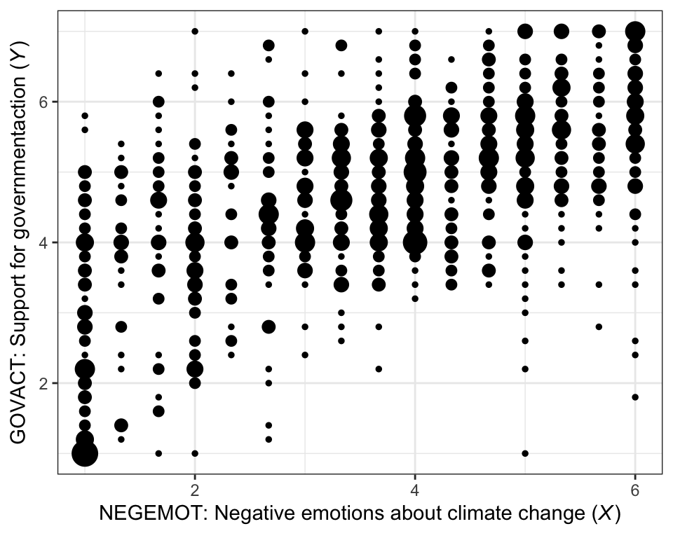

There are other ways to handle the overplotting issue, such as jittering.

glbwarm %>% 
  ggplot(aes(x = negemot, y = govact)) +
  geom_jitter(height = .05, width = .05, 
              alpha = 1/2, size = 1/3) +
  labs(x = expression(paste("NEGEMOT: Negative emotions about climate change (", italic("X"), ")")),
       y = expression(paste("GOVACT: Support for governmentaction (", italic("Y"), ")"))) +
  theme_bw()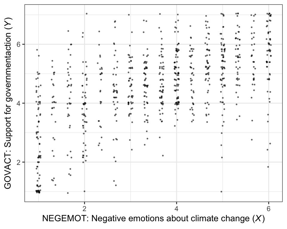

The cor() function is a simple way to compute a Pearson’s correlation coefficient.

cor(glbwarm$negemot, glbwarm$govact)
#> [1] 0.578

If you want more plentiful output, the cor.test() function returns a \(t\)-value, the degrees of freedom, the corresponding \(p\)-value and the 95% confidence intervals, in addition to the Pearson’s correlation coefficient.

cor.test(glbwarm$negemot, glbwarm$govact)
#> 
#>  Pearson's product-moment correlation
#> 
#> data:  glbwarm$negemot and glbwarm$govact
#> t = 20, df = 800, p-value <2e-16
#> alternative hypothesis: true correlation is not equal to 0
#> 95 percent confidence interval:
#>  0.530 0.622
#> sample estimates:
#>   cor 
#> 0.578

To get the Bayesian version, we’ll open our focal statistical package, Bürkner’s brms. [And I’ll briefly note that you could also do many of these analyses with other packages, such as blavaan. I just prefer brms.]

library(brms)

We’ll start simple and just use the default priors and settings, but with the addition of parallel sampling via cores = 4.

model1 <- 
  brm(data = glbwarm, family = gaussian,
      cbind(negemot, govact) ~ 1,
      chains = 4, cores = 4)

print(model1)
#>  Family: MV(gaussian, gaussian) 
#>   Links: mu = identity; sigma = identity
#>          mu = identity; sigma = identity 
#> Formula: negemot ~ 1 
#>          govact ~ 1 
#>    Data: glbwarm (Number of observations: 815) 
#> Samples: 4 chains, each with iter = 2000; warmup = 1000; thin = 1;
#>          total post-warmup samples = 4000
#> 
#> Population-Level Effects: 
#>                   Estimate Est.Error l-95% CI u-95% CI Eff.Sample Rhat
#> negemot_Intercept     3.56      0.05     3.45     3.67       3633 1.00
#> govact_Intercept      4.59      0.05     4.50     4.68       3647 1.00
#> 
#> Family Specific Parameters: 
#>                        Estimate Est.Error l-95% CI u-95% CI Eff.Sample Rhat
#> sigma_negemot              1.53      0.04     1.46     1.61       3603 1.00
#> sigma_govact               1.36      0.03     1.30     1.43       3558 1.00
#> rescor(negemot,govact)     0.58      0.02     0.53     0.62       3800 1.00
#> 
#> Samples were drawn using sampling(NUTS). For each parameter, Eff.Sample 
#> is a crude measure of effective sample size, and Rhat is the potential 
#> scale reduction factor on split chains (at convergence, Rhat = 1).

Within the brms framework, \(\sigma\) of the Gaussian likelihood is considered a family-specific parameter (e.g., there is no \(\sigma\) for the Poisson distribution). When you have an intercept-only regression model with multiple variables, the covariance among their \(\sigma\) parameters are correlations. Since our multivariate model is of two variables, we have one covariance for the \(\sigmas\)s, rescor(negemot,govact), which is our Bayesian analogue to the Pearson’s correlation.

To learn more about the multivariate syntax in brms, click here or code vignette("brms_multivariate").

But to clarify the output:

‘Estimate’ = the posterior mean, analogous to the frequentist point estimate
‘Est.Error’ = the posterior \(SD\), analogous to the frequentist standard error
‘l-95% CI’ = the lower-level of the percentile-based 95% Bayesian credible interval
‘u-95% CI’ = the upper-level of the same