12.3 Statistical inference
12.3.1 Inference about the direct effect.
We’ve already computed the 95% intervals for these. Here they are as stat_pointinterval() plots.
post %>%
  select(starts_with("direct")) %>%
  gather() %>%
  mutate(key = str_remove(key, "direct effect when W is ") %>% as.double()) %>%

  ggplot(aes(x = key, y = value, group = key)) +
  stat_pointinterval(point_interval = median_qi, .prob = c(.95, .5)) +
  coord_cartesian(xlim = c(1, 5.5)) +
  labs(x = expression(paste("Climate Change Skepticism (", italic(W), ")")),
       y = "Conditional Direct Effect of Disaster Frame on\nWillingness to Donate")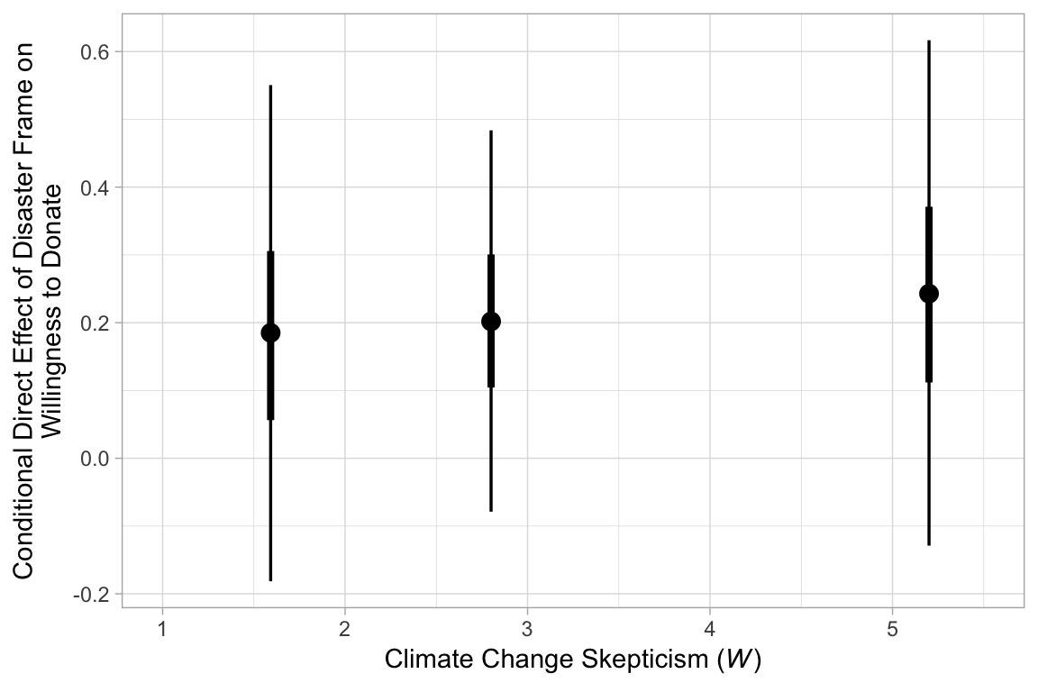
12.3.2 Inference about the indirect effect.
12.3.2.1 A statistical test of moderated mediation.
To get a sense of \(a_{3}b\), we just:
post <-
  post %>%
  mutate(a3b = `b_justify_frame:skeptic`*b_donate_justify)

post %>%
  select(a3b) %>%
  summarize(median = median(a3b),
            sd = sd(a3b),
            ll = quantile(a3b, probs = .025),
            ul = quantile(a3b, probs = .975)) %>%
  mutate_if(is.double, round, digits = 3)
## median sd ll ul
## 1 -0.182 0.055 -0.295 -0.082We might use stat_pointintervalh() to visualize \(a_{3}b\) with a coefficient plot.
post %>%
  ggplot(aes(x = a3b, y = 1)) +
  stat_pointintervalh(point_interval = median_qi, .prob = c(.95, .5)) +
  scale_y_discrete(NULL, breaks = NULL) +
  coord_cartesian(xlim = c(-.5, 0)) +
  labs(title = expression(paste("Coefficient plot for ", italic(a)[3], italic(b), " (i.e., the index of moderated mediation)")),
       x = NULL)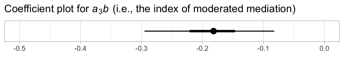
12.3.2.2 Probing moderation of mediation.
As discussed in my manuscript for Chapter 11, our Bayesian version of the JN technique should be fine because HMC does not impose the normality assumption on the parameter posteriors. In this instance, I’ll leave the JN technique plot as an exercise for the interested reader. Here we’ll just follow along with the text and pick a few points.
We computed and inspected these 95% intervals, above. Here we look at the entire densities with geom_halfeyeh().
post %>%
  select(starts_with("indirect")) %>%
  gather() %>%
  rename(`indirect effect` = value) %>%
  mutate(W = str_remove(key, "indirect effect when W is ") %>% as.double()) %>%


  ggplot(aes(x = `indirect effect`, y = W, fill = W %>% as.character())) +
  geom_halfeyeh(point_interval = median_qi, .prob = c(0.95, 0.5)) +
  scale_fill_brewer() +
  scale_y_continuous(breaks = c(1.592, 2.8, 5.2),
                     labels = c(1.6, 2.8, 5.2)) +
  coord_cartesian(xlim = -1:1) +
  theme(legend.position = "none",
        panel.grid.minor.y = element_blank())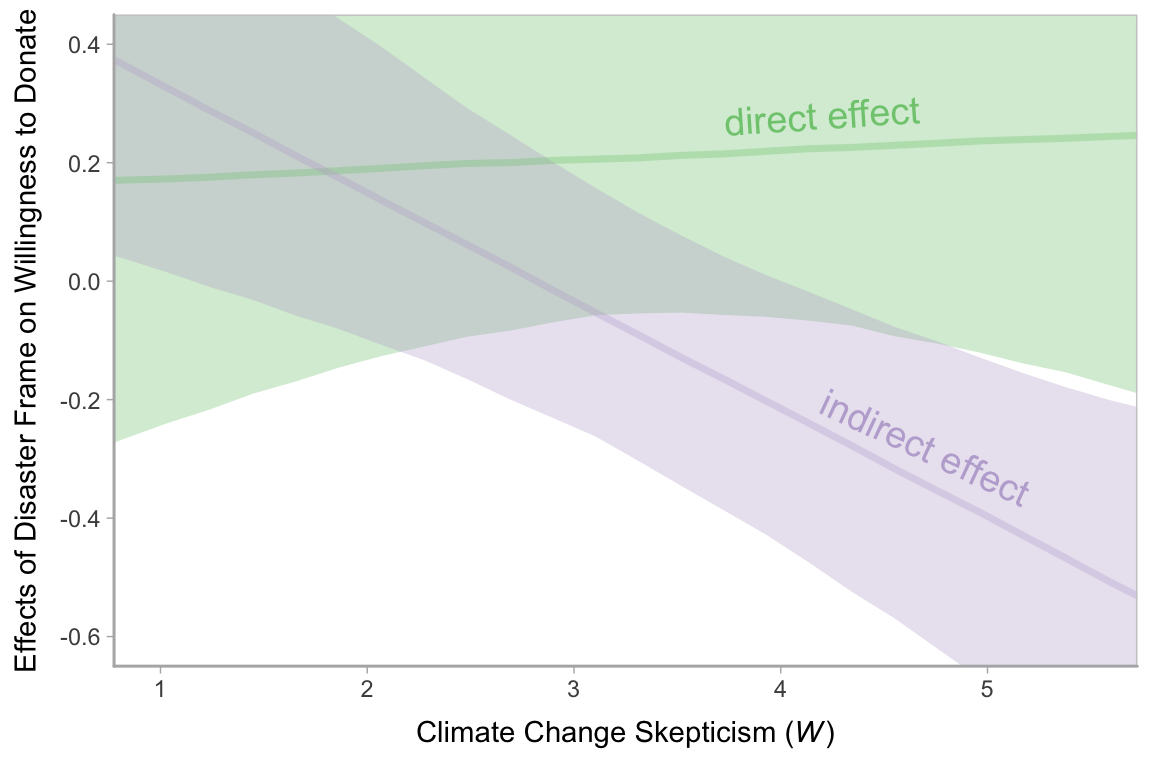
12.3.3 Pruning the model.
Fitting the model without the interaction term is just a small change to one of our formula arguments.
model4 <-
  brm(data = disaster, family = gaussian,
      bf(justify ~ 1 + frame + skeptic + frame:skeptic) +
        bf(donate ~ 1 + frame + justify + skeptic) +
        set_rescor(FALSE),
      chains = 4, cores = 4)
Here are the results.
print(model4, digits = 3)## Family: MV(gaussian, gaussian)
## Links: mu = identity; sigma = identity
## mu = identity; sigma = identity
## Formula: justify ~ 1 + frame + skeptic + frame:skeptic
## donate ~ 1 + frame + justify + skeptic
## Data: disaster (Number of observations: 211)
## Samples: 4 chains, each with iter = 2000; warmup = 1000; thin = 1;
## total post-warmup samples = 4000
##
## Population-Level Effects:
## Estimate Est.Error l-95% CI u-95% CI Eff.Sample Rhat
## justify_Intercept 2.454 0.149 2.161 2.745 3240 1.001
## donate_Intercept 7.258 0.234 6.813 7.726 4000 1.000
## justify_frame -0.565 0.219 -1.003 -0.144 2774 1.002
## justify_skeptic 0.105 0.038 0.033 0.180 3178 1.001
## justify_frame:skeptic 0.202 0.056 0.094 0.311 2568 1.003
## donate_frame 0.208 0.143 -0.071 0.488 4000 0.999
## donate_justify -0.918 0.083 -1.083 -0.759 4000 1.000
## donate_skeptic -0.037 0.037 -0.109 0.037 4000 1.000
##
## Family Specific Parameters:
## Estimate Est.Error l-95% CI u-95% CI Eff.Sample Rhat
## sigma_justify 0.818 0.040 0.744 0.900 4000 1.000
## sigma_donate 0.986 0.050 0.896 1.091 4000 1.000
##
## Samples were drawn using sampling(NUTS). For each parameter, Eff.Sample
## is a crude measure of effective sample size, and Rhat is the potential
## scale reduction factor on split chains (at convergence, Rhat = 1).Since we’re altering the model, we may as well use information criteria to compare the two versions.
loo(model3, model4)## LOOIC SE
## model3 1117.48 33.12
## model4 1115.41 33.13
## model3 - model4 2.07 0.53The difference in LOO-CV values for the two models was modest. There’s little predictive reason to choose one over the other. You could argue that model4 is simpler than model3. Since we’ve got a complex model either way, one might also consider which one was of primary theoretical interest.